adaptive fuzzy sliding mode control

Authors: Seonghyeon Jo(cpsc.seonghyeon@gmail.com)

Date: Jan 20, 2022

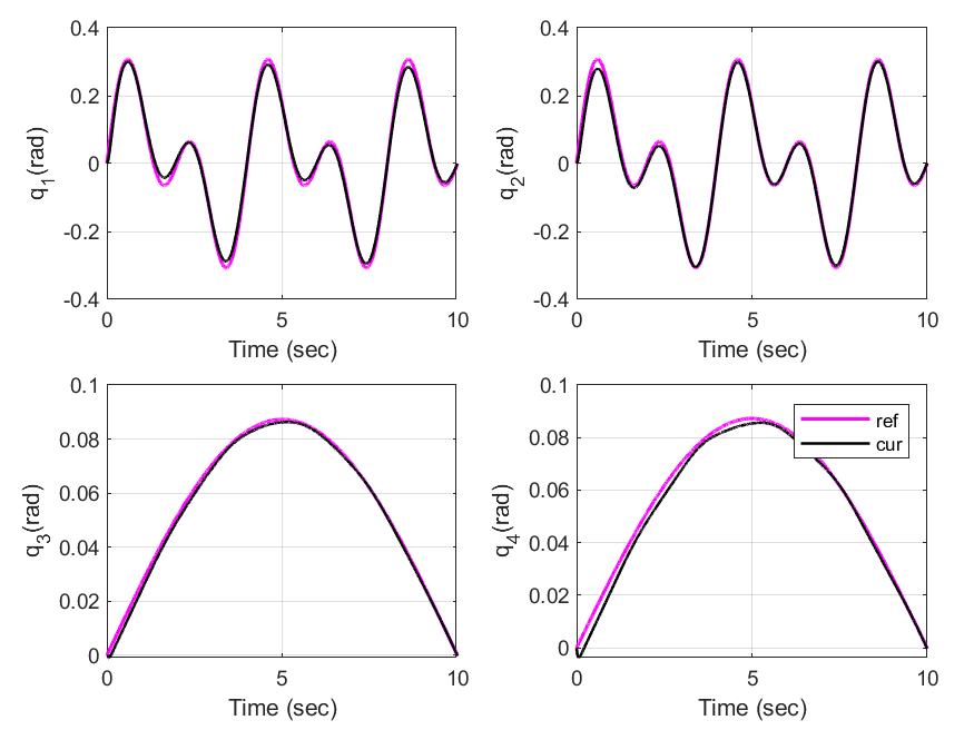
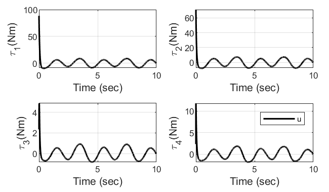
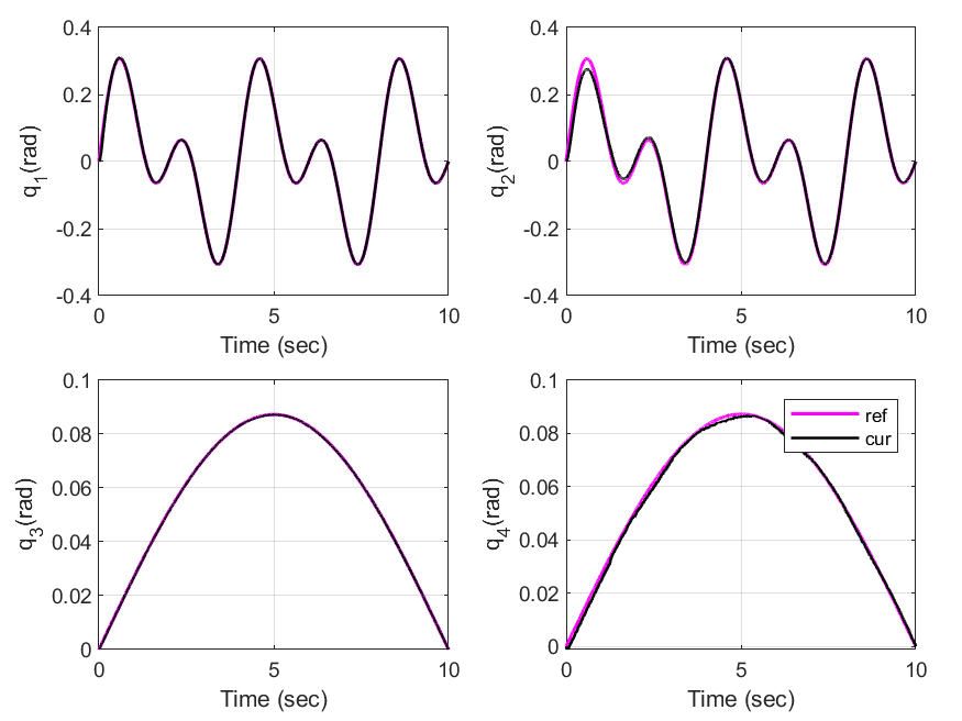
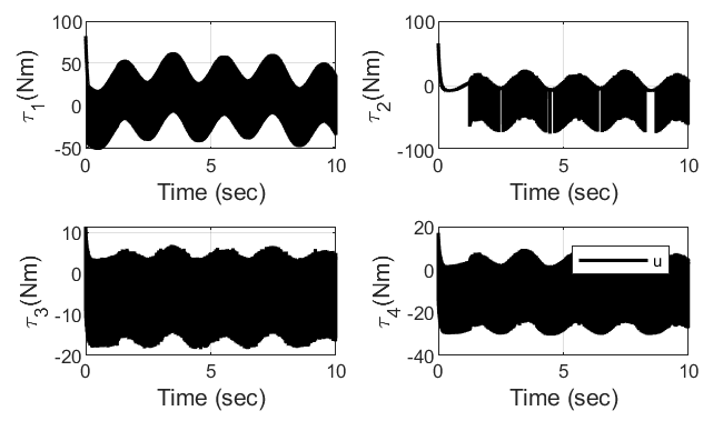
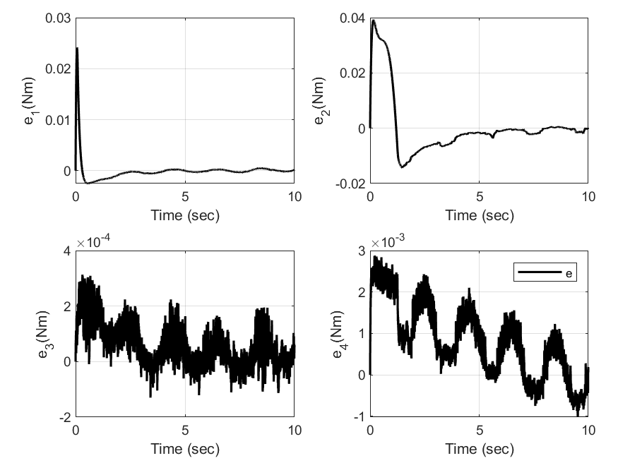
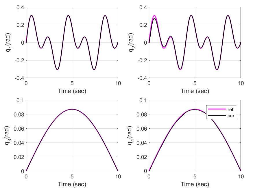
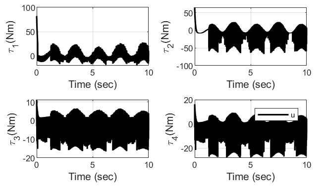
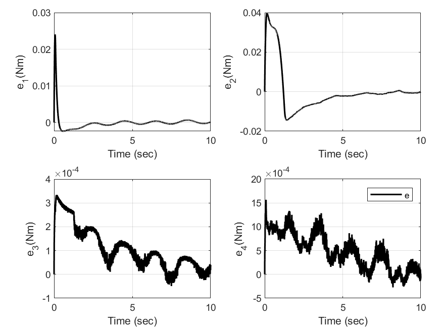
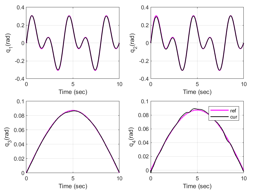
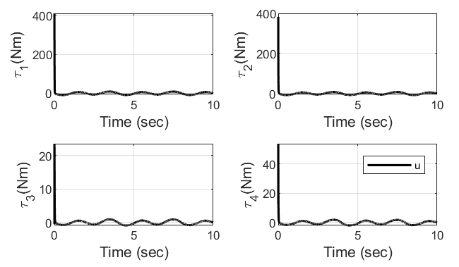
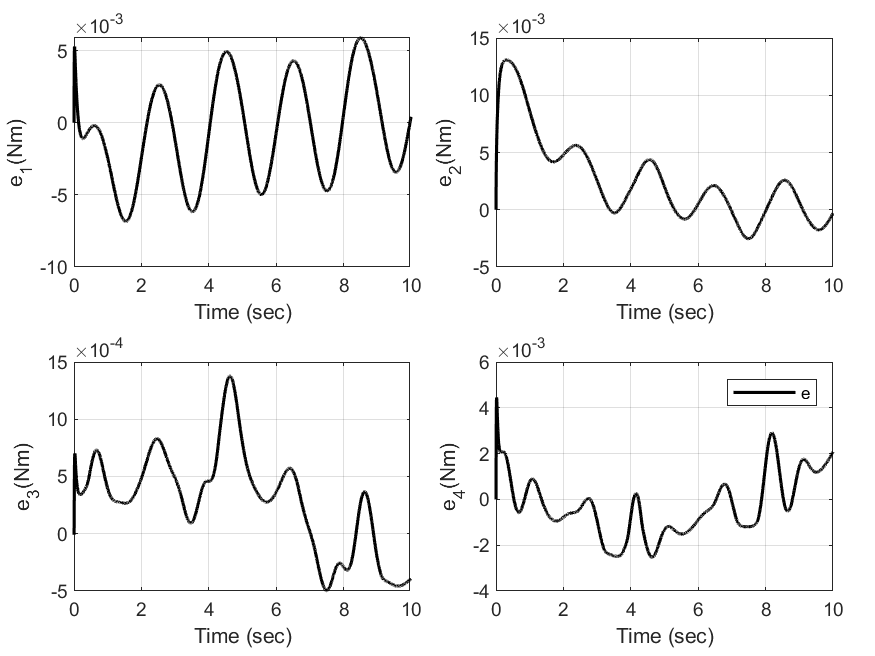
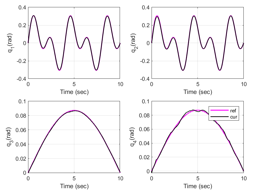
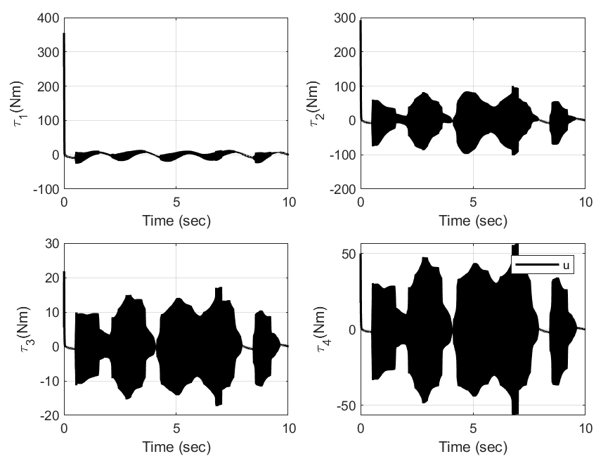
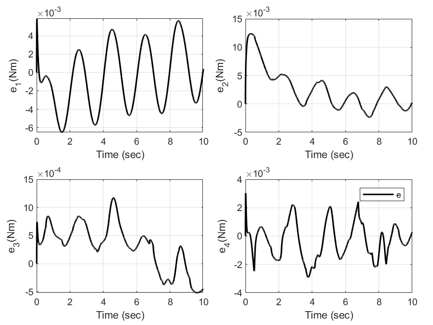
This repository is a MATLAB simulation of adaptive fuzzy sliding mode control for robot manipulator. The robot manipulator uses sawyer 4-dof manipulator and prototype 3-dof manipulator. we compare to simple PID Controller, Sliding Mode Control(SMC), Fuzzy Silding Mode Control(FSMC), Adaptive Fuzzy Sliding Mode Control(AFSMC).

"Adaptive fuzzy sliding mode control using supervisory fuzzy control for 3 DOF planar robot manipulators."

Description of robot manipulator model

In general, the dynamic of a robotic manipulator can be expressed as follows: $\M(\q)\ddot{\q} + \C(\q,\dot{\q})\dot{\q}+\G(\q)+\F(\dot{\q}) =\boldsymbol\tau + \boldsymbol\tau_d$ where $\q, \dot{\q}, \ddot{\q}, \boldsymbol\tau, \boldsymbol\tau_d \in \mathcal{R}^{n}$ denote the joint position vector, velocity vector, acceleration, the vector of control torques, and the vector of disturbance torques, respectively, and $\M\in\mathcal{R}^{n\times n}$ denotes the symmetric positive definite inertia matrix, $\C \in \mathcal{R}^{n\times n}$ denotes the Coriolis matrix, $\G \in \mathcal{R}^{n}$ denotes the gravity vector and $\F \in \mathcal{R}^{n}$ is the friction matrix.

Multiplying $M^{-1}(q)$ by both sides in Equation (1), we have

$\ddot{\q}=-\M^{-1}(\q)(\C(\q,\dot{\q})\dot{\q}+\G(\q)+\F(\dot{\q})-\boldsymbol\tau-\boldsymbol\tau_d )$

The sliding proportional-integral-derivative PID surface in the space of tracking error can be defined as:

$\begin{align*} \s(t)&=K_{p}\e(t)+K_{i}\int{\e}(\tau)d\tau+K_{d}\dot{\e}(t) \end{align*}$

where kp is positive proportional gain matrix, ki is positive integral gain matrix, kd is positive derivative gain.

Take the derivative of sliding surface with respect to time, then

$\begin{align*} \dot{\s}(t) &= K_p \dot{\e}(t) + K_i \e(t)+ K_{d}\ddot{\e}(t)\\ &= K_p \dot{\e}(t) + K_i \e(t)+K_d (\ddot{\q}_d+\M^{-1}(\q)(\C(\q,\dot{\q})\dot{\q}+\G(\q)+\F(\dot{\q})-\boldsymbol\tau-\boldsymbol\tau_d)\\ \end{align*}$

The control effort being derived as the solution of s˙(t) = 0 without considering uncertainty (d(t) = 0) is to achieve the desired performance under nominal model, and it is referred to as equivalent control effort , represented by ueq(t)

$\begin{align*} \u_{eq}= (K_d\M^{-1}(\q))^{-1}(K_p \dot{\e} + K_i \e+K_d (\ddot{\q}_d+\M^{-1}(\q)(\C(\q,\dot{\q})\dot{\q}+\G(\q)+\F(\dot{\q}))) \end{align*}$

sawyer 4-dof manipulator

RMSE

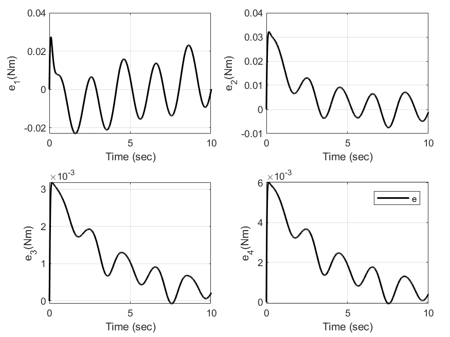
Method	joint 1	joint 2	joint 3	joint 4	sum
PID	0.0394	0.0339	0.0044	0.0083	0.0860
SMC-SIGN	0.0078	0.0349	0.0003	0.0039	0.0469
SMC-SAT	0.0078	0.0358	0.0004	0.0019	0.0460
FSMC	0.0111	0.0146	0.0017	0.0043	0.0317
AFSMC	0.0105	0.0141	0.0013	0.0042	0.0301