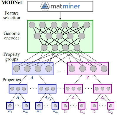
This repository contains the python package implementing the Material Optimal Descriptor Network (MODNet). It is a supervised machine learning framework for learning material properties from the crystal structure. The framework is well suited for limited datasets and can be used for learning multiple properties together by using joint transfer learning.
This repository also contains two pretrained models that can be used for predicting the refractive index and vibrational thermodynamics for any crystal structure.
See the MODNet paper for more details:
Machine learning materials properties for small datasets, De Breuck et al. (2020), arXiv:2004.14766.
MODNet can be installed via pip:
pip install modnetThe MODNet package is built around two classes: MODData and MODNetModel.
The usual workflow is as follows:
from modnet.preprocessing import MODData
from modnet.models import MODNetModel

# Creating MODData
data = MODData(structures,targets)
data.featurize()
data.feature_selection(n=1000)

# Creating MODNetModel
model = MODNetModel(target_hierarchy,weights,num_neurons=[[256],[64,64],[32]])
model.fit(data)

# Predicting on unlabeled data
data_to_predict = MODData(new_structures)
data_to_predict.featurize()
df_predictions = model.predict(data_to_predict) # returns dataframe containing the prediction on new_structures
Example notebooks can be found in the example_notebooks directory.
Two pretrained models are provided in pretrained/:
- Refractive index
- Vibrational thermodynamics
Download this directory localy to path/to/pretrained/. Pretrained models can then be used as follows:
from modnet.models import MODNetModel

model = MODNetModel.load('path/to/pretrained/refractive_index')
# or MODNetModel.load('path/to/pretrained/vib_thermo')Three MODDatas are provided in moddata/:
- Refractive index
- Vibrational thermodynamics
- Formation energy on Materials Project (June 2018)
Download this directory localy to path/to/moddata/. These can then be used as follows:
from modnet.preprocessing import MODData

data_MP = MODData.load('path/to/moddata/MP_2018.6')
The latter MODData (MP_2018.6) is very usefull for predicting a learned property on all structures from the Materials Project:
predictions_on_MP = model.predict(data_MP)The two main classes, MODData and MODNetModel, are detailed here.
A MODData instance is used for representing a particular dataset. It contains a list of structures and corresponding properties:
from modnet.preprocessing import MODData

data = MODData(structures, targets, target_names=None, mpids=None)
Arguments:
structures (List): List of pymatgen Structures.targets (List): optional List of targets corresponding to each structure. When learning on multiple targets this is a ndarray where each column corresponds to a target, i.e. of shape (n_materials,n_targets).target_names (Iterable)(optional): Iterable (e.g list) of names corresponding to the properties. E.g.['S_300K','S_800K',...]or['refractive_index']for single target learning. These names are used when building the model.structure_ids (Iterable)(optional): If the list of structures (structures) are from the Materials Project, you can specify the corresponding mpids by providing an Iterable of mpids:['mp-149','mp-166',...]. This will enable fast featurization (see further).
The next step is to create the features:
data.featurize(fast=False,db_file='feature_database.pkl')Arguments:
fast (Boolean)(optional): If set to True, the algorithm will use the pre-computed features from a database instead of computing them again from scratch. This is recommended (and only possible) when using structures from the Materials Project. Note that the mpids should be provided in the MODData.db_file (Boolean)(optional): When setting fast to True, you also need to provide this argument. Download the file at this figshare link, unzip it, then set the local path to this file as argument.
Finally, the optimal features are computed:
data.feature_selection(n=300)Arguments:
n(optional): Number of optimal features to compute, i.e. the n first ranked features are computed. When set to -1, all features are ranked (recommended, but can take time).
The MODData can be saved,
data.save('path/dataname')and loaded for later usage:
from modnet.preprocessing import MODData

data = MODData.load('path/dataname')
Both the save and load methods use pandas .read_pickle(...) and .load_pickle(...) which will try to compress/decompress files according to their file extensions (e.g. ".zip", ".tgz" and ".bz2".
Dataframes for features, targets and other data can be accessed trough the following methods:
# dataframe containing the structures
data.get_structure_df()

# dataframe containing the targets
data.get_target_df()

# dataframe containing the features
data.get_featurized_df()

# List of the optimal features, in ranked order
data.get_optimal_descriptors()

# get_featurized_df limited to the best features
data.get_optimal_df()The model is created by a MODNetModel instance:
from modnet.models import MODNetModel

model = MODNetModel(targets,weights,num_neurons=[[64],[32],[16],[16]], n_feat=300, loss='mse',act='relu')
Arguments:
-
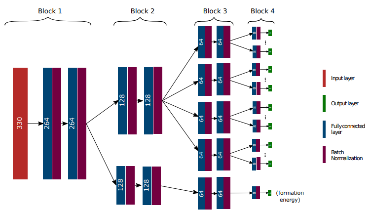
targets (List): Specifies how the different targets are organized in the architecture. It is a list of lists of lists, representing the three modular last levels: block 2, 3 and 4 (see Figure 2). Each block gathers properties, which are put inside the same list. For exmaple, in Figure 2, this is [[['S_5,...,S_800'],['U_5,...,U_800'],['C_v_5,...,C_v_800'],['H_5,...,H_800']],[['formation_energy']]]. The same names as given inMODDatashould be used. -
weights (Dictionary): A dictionary where each key is a property name and the value the corresponding weight to be used in the loss function. The weights are used to scale the different outputs such that the balance between the properties is conserved when training. For example, {'S_5':0.01, 'formation_energy:1'}. -
num_neurons (List)(optional): Number of neurons as well as the number of layers to be used in the neural network. List of three lists. Each inner list gives respectively the succesive number of neurons of the blocks 2, 3 and 4. For example, in Figure 2, this is given by [[128,128],[64,64],[8]]. -
n_feat (int)(optional): Number of optimal features to be used in the model. In Figure 2, this is 330. -
loss (String)(optional): Loss function of the neural network, see Keras API. -
act (String)(optional): Activation function used in the neural network, see Keras API.
The model is then fitted on the data:
model.fit(data, val_fraction = 0.0, val_key = None, lr=0.001, epochs = 200, batch_size = 128, xscale='minmax'):Arguments:
val_fraction (float)(optional): Validation fraction to be used while training.val_key (String)(optional): The name of the property used for printing validation MAE. When multiple properties are learned (e.g.['formation energy', 'refractive_index', 'entropy']), setting the key_val (e.g.key_val = 'entropy') will only print the MAE of this property for each epoch.lr (float)(optional): Learning rate.epochs (int)(optional): Number of epochs.batch_size (int)(optional): Batch size.xscale (String)(optional): Scaling of the features. Possible values:'minmax'or'standard'.
You can save and load the model for later usage:
model.save('path/modelname')from modnet.models import MODNetModel
MODNetModel.load('path/modelname')Prediction is done by first creating a MODData instance on the new data:
data_to_predict = MODData(structures, mpids = df.index) # Adding mpids is a good idea for fast featurization, but not necessary.
data_to_predict.featurize(fast=True)
and then using the predict method:
df_predictions = model.predict(data_to_predict)A dataframe containing the predictions is returned.
This software is written by Pierre-Paul De Breuck
MODNet is released under the MIT License.


