Pixel-Wise T-Test

A New Algorithm for Battle Damage Detection using Sentinel-1 Imagery

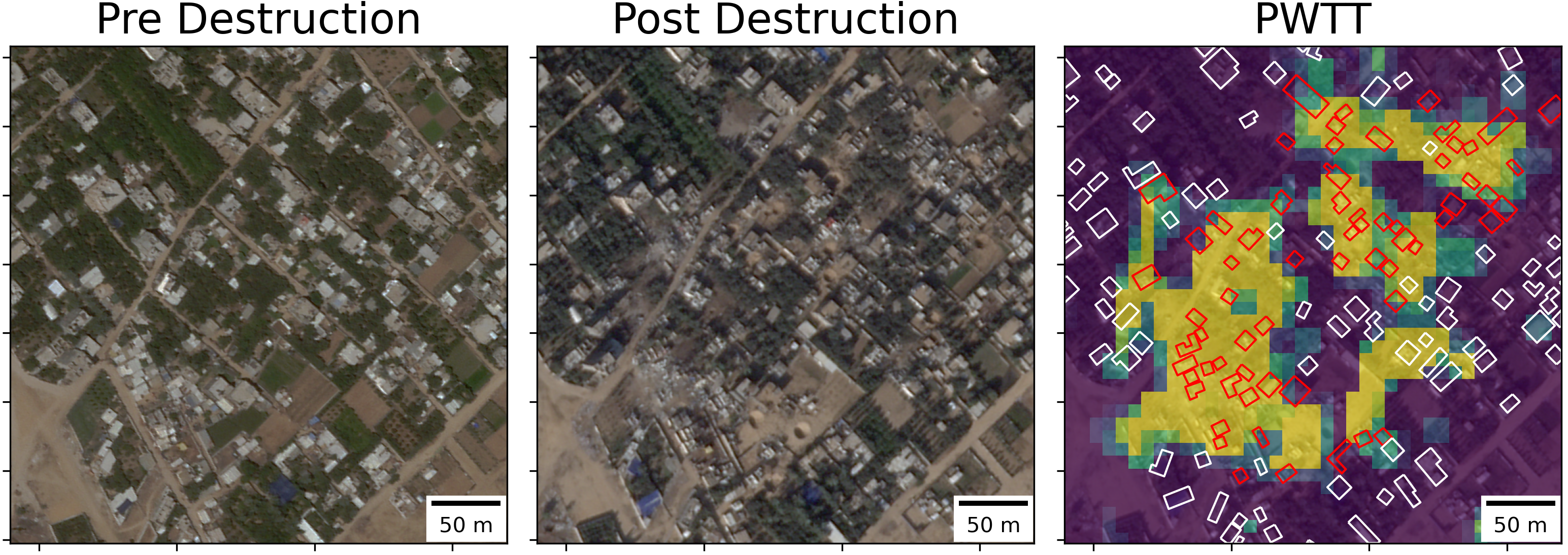
The generation of public information regarding buildings damaged by conflict has become particularly important in the context of recent, highly destructive wars in Gaza and Ukraine. This paper develops the Pixelwise T-Test (PWTT), a new algorithm for open-access battle damage estimation that is accurate, lightweight, and generalizable. The PWTT addresses many of the problems associated with expense, coverage consistency, and domain shift that affect deep-learning based approaches to building damage detection, and outperforms the state of the art deep learning model on unseen areas.

How it Works

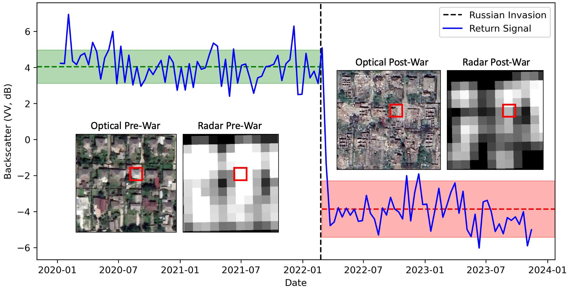
The PWTT utilizes Synthetic Aperture Radar imagery from the Sentinel-1 satellite. The figure below demonstrates the change in backscatter amplitude (i.e., the "loudness" of the signal's echo) for a destroyed building in Mariupol, Ukraine, before and after its destruction. The corresponding Sentinel-1 pixel has a low standard deviation in both the pre-and post-war periods, but experiences a large change in mean amplitude. The T-Test is a simple signal-to-noise ratio that measures the difference between the means of two samples adjusted by the standard deviation within each sample.

The green dashed line and shaded area represent the pixel's mean backscatter amplitude $\pm$ 1 standard deviation prior to the invasion, while the red line and shaded area represent these statistics following the building's destruction.

Python Quickstart

First, clone the repository and navigate to the code directory

!git clone https://github.com/oballinger/PWTT
!cd PWTT/code

Then, import the Google Earth Engine python API and authenticate using your credentials and cloud project name.

import ee
import pwtt

project_name='<YOUR PROJECT NAME>'
ee.Authenticate()
ee.Initialize(project=project_name)

finally, the PWTT can be deployed in one line of code. The example below conducts a damage assessment over Gaza for July 2024.

gaza = ee.Geometry.Rectangle([34.21,31.21,34.57,31.60])

pwtt.filter_s1(aoi=gaza, # the area of interest as a bounding box
                   war_start='2023-10-10', # the start of the war
                   inference_start='2024-07-01', # the beginning of the inference window
                   pre_interval=12, # the number of months before the war to use as a reference period 
                   post_interval=1, # the number of months after the war to use as an inference period 
                   viz=True) # visualize the results

By simply modifying the location, war_start date and inference_start dates, damage assessment can be carried out on a new area; below is another example for Bakhmut, Ukraine:

bakhmut = ee.Geometry.Rectangle([37.949421, 48.556181, 38.043834, 48.621584])

pwtt.filter_s1(aoi=bakhmut,
                   war_start='2022-02-22',
                   inference_start='2024-07-01',
                   pre_interval=12,
                   post_interval=1,
                   viz=True)

Validation Data

Accuracy assessments are carried out using an original dataset of 700,500 annotated building footprints, spanning 12 cities in four different countries. This dataset was compiled by spatially joining damage annotations from the United Nations Satellite Centre (UNOSAT) with data on building footprints. The dataset can be downloaded here.

Benchmark Dataset

Country	City	Footprints	Percent Damaged	Annotation Date
Palestine	Gaza	220160	57.21%	2024-05-03
Ukraine	Lysychansk	22280	7.77%	2022-09-21
Ukraine	S'odonetsk	7085	25.43%	2022-07-27
Ukraine	Rubizhne	9905	33.81%	2022-07-09
Ukraine	Kharkiv	122590	0.91%	2022-06-15
Ukraine	Mariupol	20481	32.57%	2022-05-12
Ukraine	Hostomel	4728	14.11%	2022-03-31
Ukraine	Irpin	7917	11.56%	2022-03-31
Ukraine	Chernihiv	33733	3.36%	2022-03-22
Syria	Raqqa	26728	45.78%	2017-10-21
Syria	Aleppo	73634	31.45%	2016-09-18
Iraq	Mosul	151259	11.59%	2017-08-04

Building footprint data is sourced from the Microsoft Building Footprints dataset, which consists of over 1 billion building footprints derived from high resolution satellite imagery around the world. A building footprint is labeled as damaged if it intersects with a UNOSAT damage annotation point, and labeled undamaged otherwise. UNOSAT annotations are generated manually on the basis of high resolution optical satellite imagery.

Accuracy Assessment

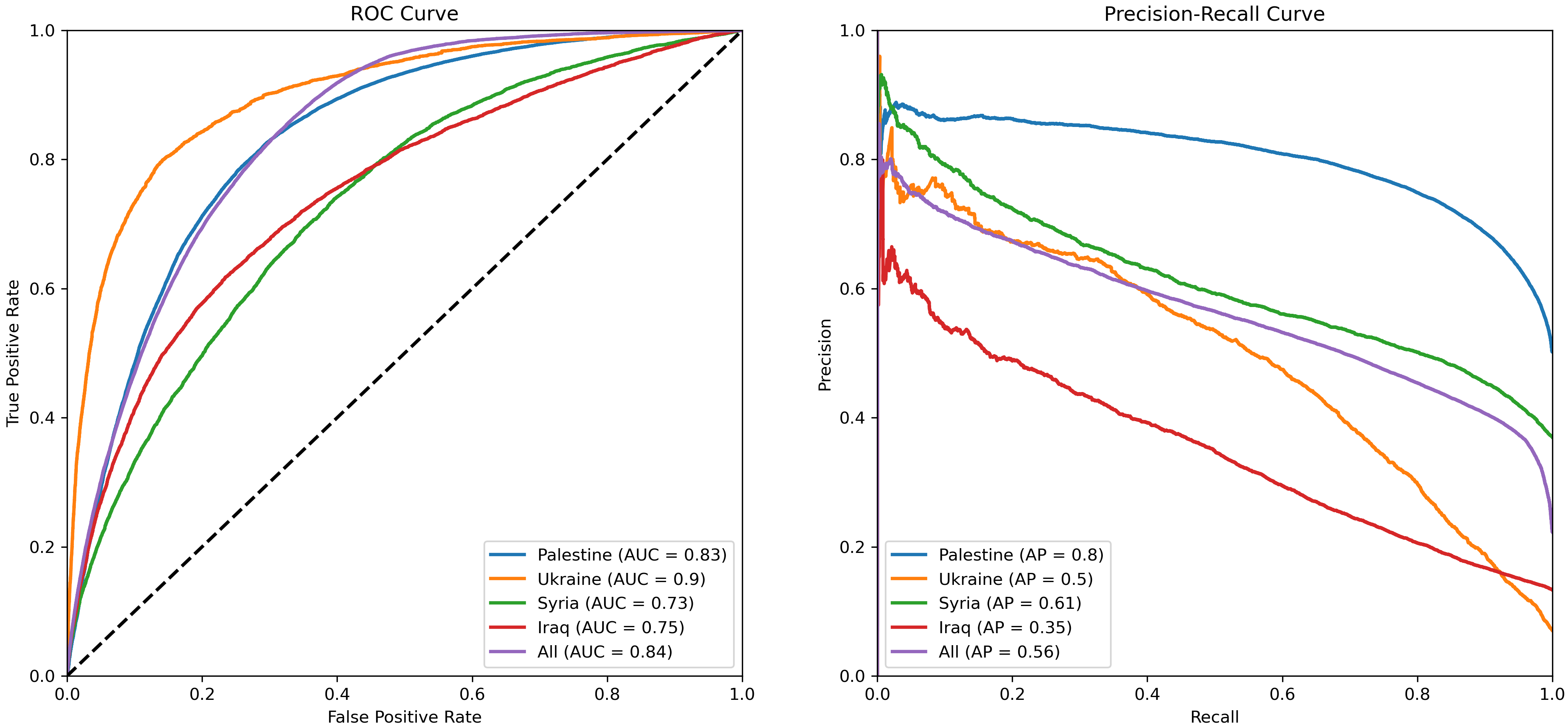
The table below reports the accuracy statistics for the PWTT algorithm in 12 cities, assessed using the benchmark dataset above.

City	AUC	F1	Precision	Recall	N
Gaza	83.13	78.72	71.68	87.3	220160
Lysychansk	77.5	52.47	46.24	60.64	22280
S'odonetsk	69.36	64.98	50.28	91.84	7085
Rubizhne	77.72	67.5	68.55	66.48	9905
Kharkiv	78.66	27.72	25.03	31.06	122590
Mariupol	70.48	71.58	61.38	85.84	20481
Irpin	83.94	59.41	54.53	65.24	7917
Hostomel	86.25	73.49	67.66	80.41	4728
Chernihiv	84.65	46.92	53.07	42.05	33733
Raqqa	76.38	75.22	66.27	86.95	26728
Mosul	76.16	42.91	39.16	47.46	151259
Aleppo	74.42	65.15	52.71	85.27	73634
All	82.0	60.92	51.22	75.16	700500

Reciever-Operating Characteristic (ROC) curves for each country are also provided below.