Cartpole system playground
This repo contains a simulation of a cartpole system (pendulum on a trolley) with various control engineering stuff. It's meant to refresh a few concepts and test capabilities of Julia.
Simulated system is governed by the following equations of motion:
where:
- position and speed of the cart (trolley), positive to the right
- angle and angular velocity of the pole (pendulum), 0 at the bottom position, positive counter-clockwise
- mass of the cart and the pole
- friction coefficients of the cart (and ground) and the pole (and cart)
- the length of the pole
- force applied to the cart, positive to the right
Developed with Julia version 1.7.2. Start the session with:
include("main.jl")Simple simulation from initial conditions
Function simulate_cartpole() to simulate the system from initial conditions (stored in CartPoleState) with given parameters (stored in CartPoleParams struct). Examples:
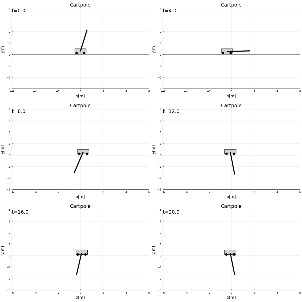
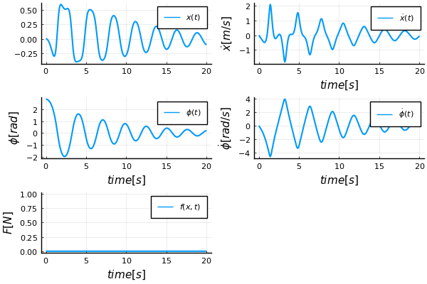
Unforced:
cp_params = CartPoleParams(
    1.0, 0.5,   # w, h
    1.0, 0.3,   # mt, mp
    2.0,        # L
    0.2, 0.2    # bt, bp
)
init_state = CartPoleState(0.0, 0.0, pi - 0.3, 0.0)
diffeq_sol, saved_values = simulate_cartpole(cp_par, init_state, (x,t) -> 0.0, (0.0, 20.0), 0.01)
plot_sol_force(diffeq_sol, saved_values; dest_name = "simulation_unforced.png")
# to create also the gif
gif_sol(sol, CartPole(cp_params, init_state); dest_name = "simulation_unforced.gif")
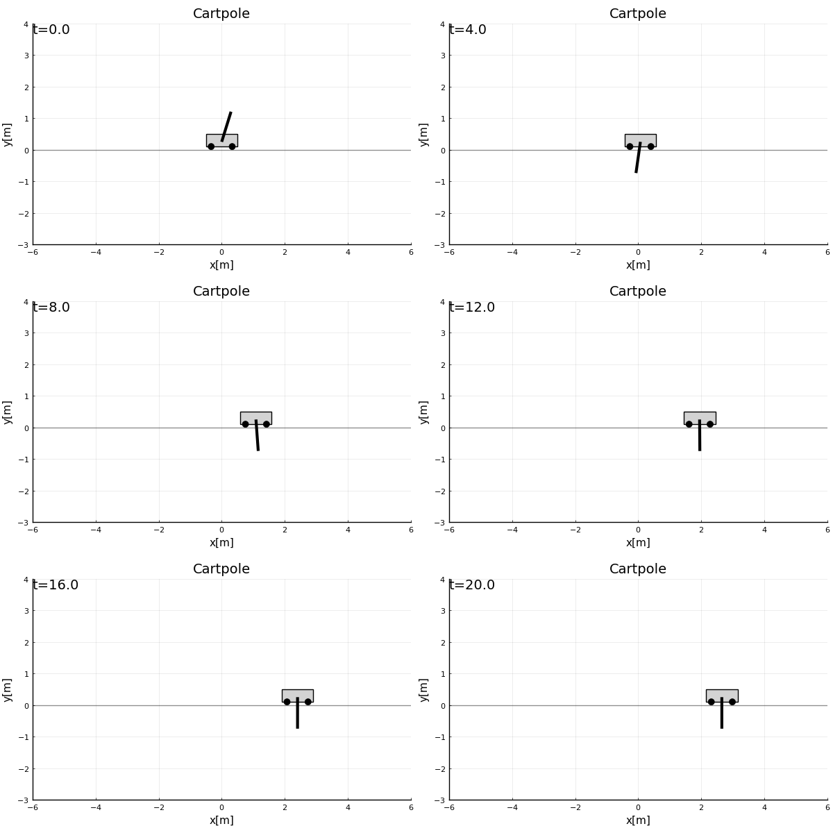
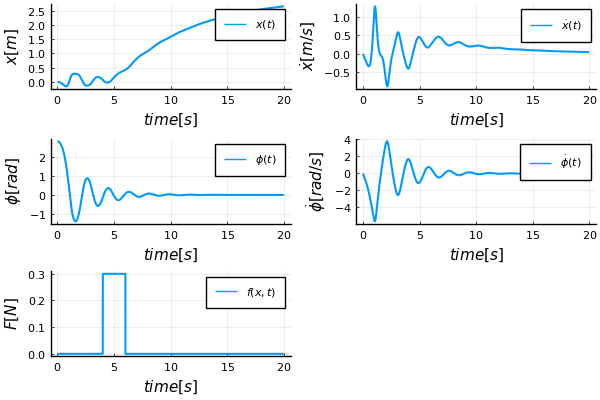
With some force applied and shorter pole:
cp_params = CartPoleParams(
    1.0, 0.5,   # w, h
    1.0, 0.3,   # mt, mp
    1.0,        # L
    0.2, 0.2    # bt, bp
)
init_state = CartPoleState(pi-0.3)  # convenient state ctor
f(x, t) = f_step(x, t; t_step_begin = 4, t_step_end = 6, weight = 0.3)
diffeq_sol, saved_values = simulate_cartpole(cp_params, init_state, f, (0.0, 20.0), 0.01)
plot_sol_force(diffeq_sol, saved_values; dest_name = "simulation_forced.png")
Estimations
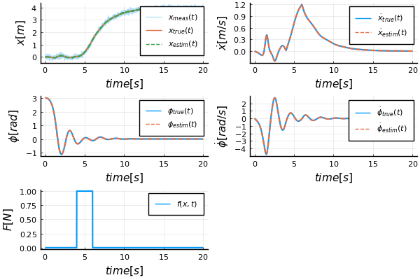
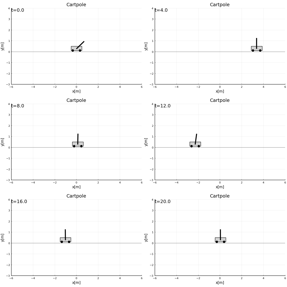
Estimation of all 4 states from a single noisy measurement of position x. The estimates are computed online via SavingCallback of the DifferentialEquations package, not offline from saved data as is usually done in examples. IMHO, online calculation is easier to understand and is closer to real application. A callback is chosen directly in the main function. The following callback estimators are implemented:
- Luenberger observer
- Linear Kalman Filter
- Extended Kalman Filter
cp_params = CartPoleParams()
init_state = CartPoleState(pi-0.1)
main_estimator_cb(cp_params, init_state; make_plot=true)
LQR control
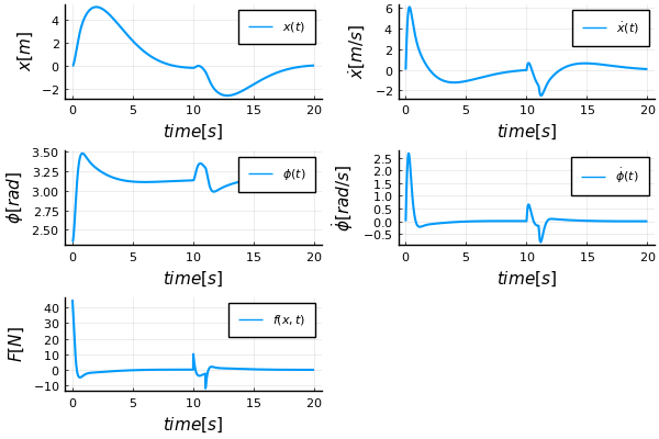
ControlSystems package is used to compute optimal gain matrix using lqr function. Example of recovery from bad initial position and subsequent push at time 10s:
cp_params = CartPoleParams()
init_state = CartPoleState(pi-0.1)
main_LQR(cp_params, init_state; make_plot=true)
Swing-up maneuver
Using nonlinear optimization
JuMP package is used to implement direct collocation method in src/swingup_optim.jl. Open loop control sequence is generated, LQR takes over near the top. A nice material for collocation methods is in An Introduction to Trajectory Optimization: How to Do Your Own Direct Collocation by Matthew Kelly.
Cost function is the sum of squares of control inputs. Constraints comprise of box constraints on states and inputs and constraints on collocation points. Initial guess is trivial: straight line from the initial to the final state.
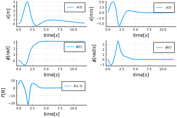
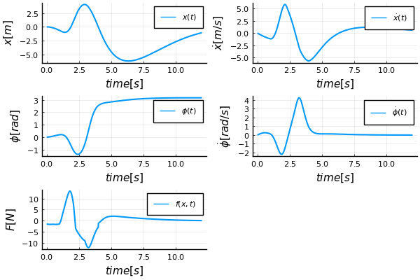
Using reinforcement learning
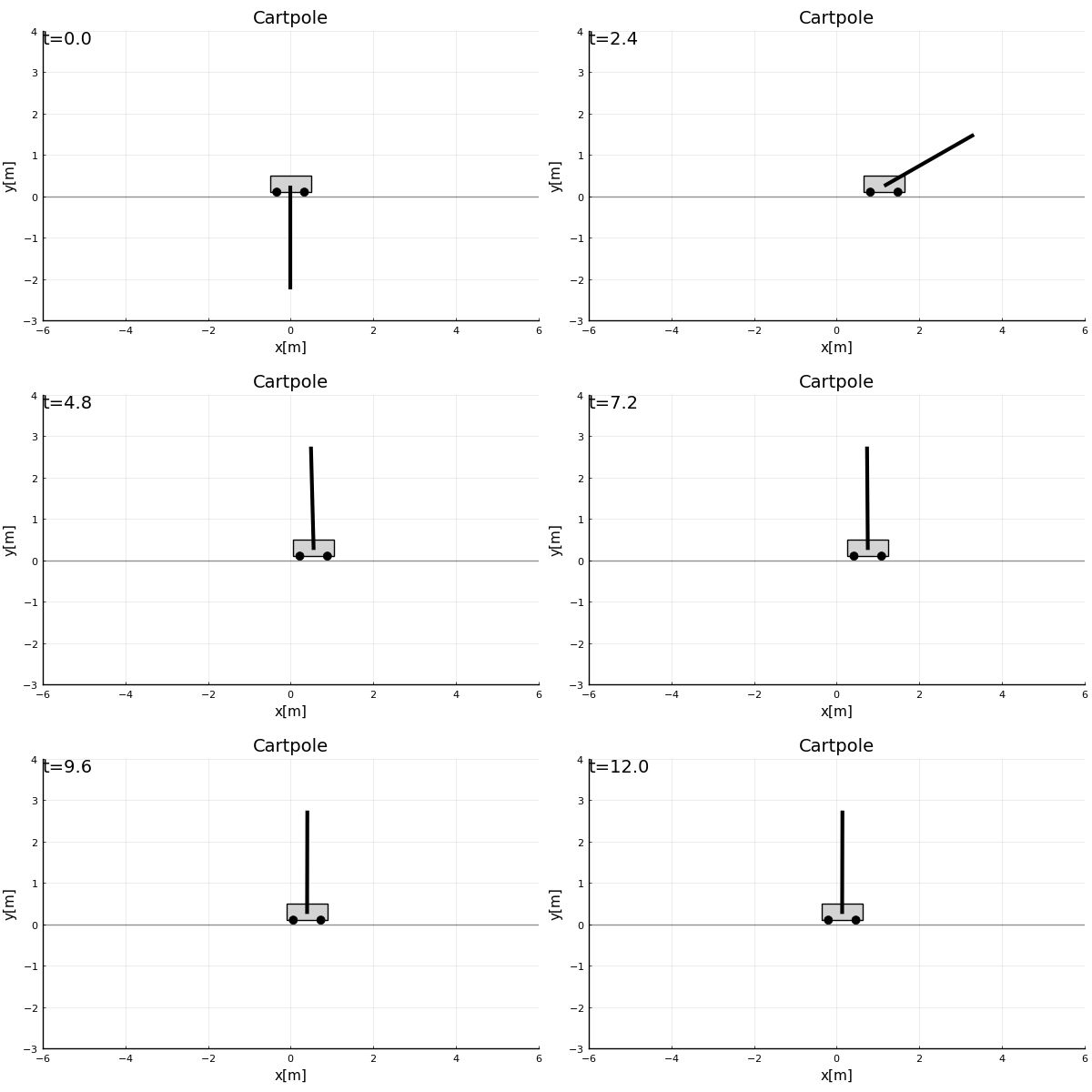
Neural network with 4 inputs, 1 hidden layer and 1 output is trained using a cost function. DiffEqFlux package does the work. Feedback law using neural network is produced and LQR takes over near the top. The code in src/swingup_rl.jl was highly inspired by this Medium post by Paul Shen
By trial and error, the following loss function had the best results. It's a weighted sum of end states plus sum of control inputs along the way:
To reproduce the graph below, write the following:
cp_par = CartPoleParams()
init_state = CartPoleState()

# read the weights for neural net
nn_par = read_nn_params_json("assets/rl_ctrl_2022-04-23_16:30:10.json")
# simulate and produce plot
main_swingup_rl(cp_par, init_state, make_plot=true, nn_params=nn_par)
To train with different cost function or other parameters just exclude the nn_params argument, function will return trained net:
nn_trained = main_swingup_rl(cp_par, init_state, make_plot=true)

# to reuse:
main_swingup_rl(cp_par, init_state, make_plot=true, nn_params = nn_trained.u)
I found it very hard to pick the right cost function to do the job and not end up with something ridiculous, here are some failed attempts :D
