A challenge on mapping pseudo altimetric data on a QG model created by Datlas and MEOM-IGE.
This repository contains codes and sample notebooks for downloading and processing the SSH QG mapping data challenge.
After several altimetric mapping challenges have been proposed to the oceanographic community (see Acknowledgment), the goal of this simplified altimetric mapping data challenge is to open a new entry point for people from other communities to play and bring their outside knowlegde to this oceanographic problem.
The goal is to investigate how to best reconstruct sequences of sea surface height (SSH) maps from partial satellite altimetric observations. The end goal is to have efficient methods that are able to extrapolate information from the partial (in time and space) satellite data in order to generate fully resolved maps of the ocean surface at all time. In this OSSE experimental context -- i.e. where we know the underlying "true" fields we want to reconstruct -- the methods' performances are assessed by directly comparing the methods' reconstructed fields to the "true" fields in terms of point-wise difference of SSH and its corresponding velocities, spectral energy distribution ... (see Diagnostics).
To simplify the realistic altimetric problem, the proposed DC is set using an idealized dynamic: a one layer and a half quasi-geostrophic motions (see for instance Ubelmann et al., 2015) which can mimic the actual ocean surface dynamics in certain geographic regions but is much simpler than the global four dimensional ocean dynamics.
The DC is composed of three set of observations of increasing realism:
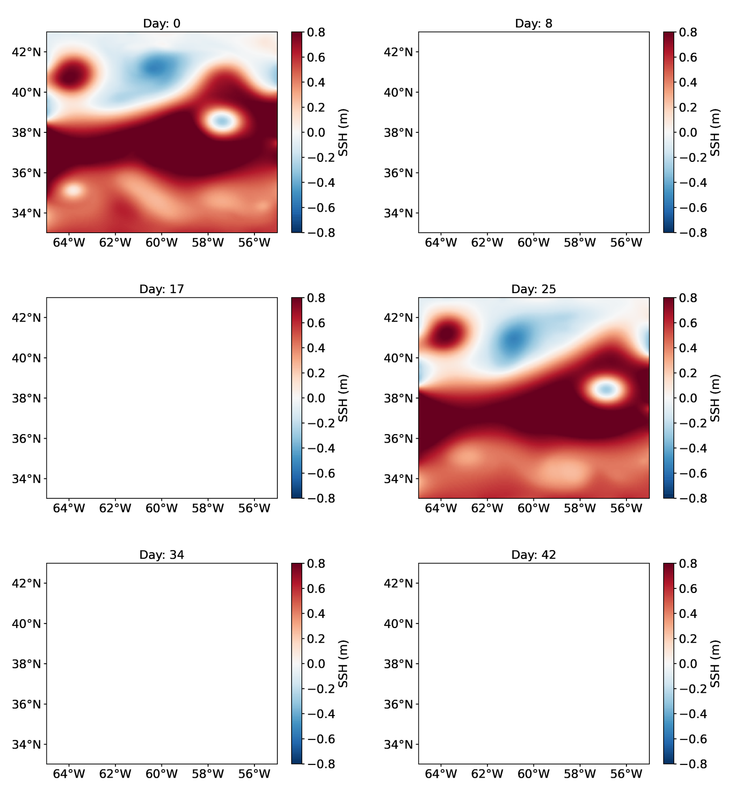
- Managing observations sparse in time: the Full field observations (A) set up consists in observing the full SSH fields of "our quasi-geostrophic ocean" every 5 day ;
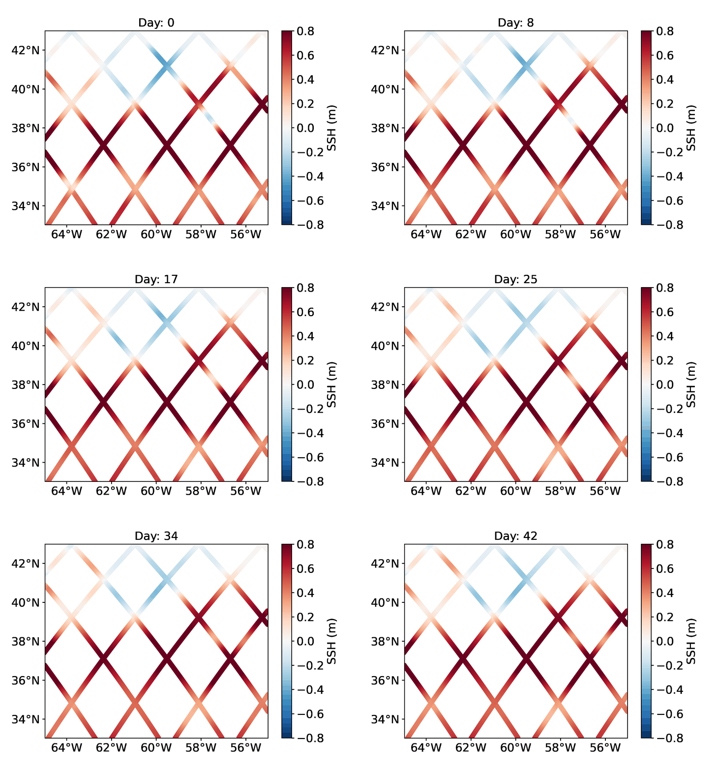
- Managing observations sparse in space: the Everyday jason1 observations (B) set up consists in observing pseudo SSH data similar to the Nadir-altimeter Jason1 data (as it would have seen the ocean over 42 days) but providing a one-dimensional look of "our quasi-geostrophic ocean" SSH every day ;
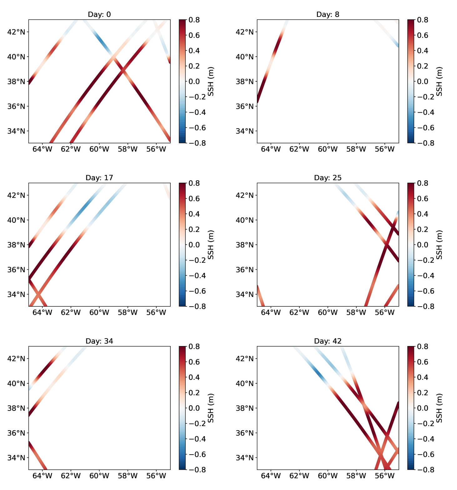
- Managing realistic observations: the Realistic observations (C) set up consists in observing "our quasi-geostrophic ocean" with similar space and time observation density as a constellation of 4 Nadir satellites (Envisat, Jason1, Geosat2 and Topex-Poseidon).
A baseline reconstruction method is provided (see below) and the practical goal of the challenge is to beat this baseline according to scores also described below and in Jupyter notebooks.
The reference simulation is a 1.5 layer quasi-geostrophic simulation generated using the model described in Ubelmann et al. (2015). The run can be downloaded from dc_qg_eval (see Download the data section below).
| True SSH |
|---|
 |
A) Managing observations sparse in time: Full field observations set up
The first set up provides observations of the full SSH fields every 5 day:
| True SSH | Full field observations (A) |
|---|---|
 |
 |
B) Managing observations sparse in space: Everyday jason1 observations set up
The second set up provides observations of one-dimensional Jason1-like SSH data (corresponding to the full 42 day availability of that satellite data) but available every day:
| True SSH | Everyday jason1 observations (B) |
|---|---|
 |
 |
C) Managing realistic observations: Realistic observations set up
The third set up provides observations of one-dimensional Nadir-like SSH data from a constellation of 4 Nadir satellites (Envisat, Jason1, Geosat2 and Topex-Poseidon):
| True SSH | Realistic observations (C) |
|---|---|
 |
 |
Understanding the data
A notebook that documents and illustrates the data is available: understand_the_data.ipyn
The baseline mapping method is optimal interpolation (OI), in the spirit of the present-day standard for DUACS products provided by AVISO. OI is implemented in the perform_the_baseline Jupyter notebook. The SSH reconstructions are saved as a NetCDF file in the results directory. The content of this directory is git-ignored so you will have to run it yourself if you want later want to run evaluate_the_baseline, for instance.
The evaluation of the mapping methods is based on the comparison of the SSH reconstructions with the reference dataset. It includes two scores, one based on the Root-Mean-Square Error (RMSE), the other based on Fourier wavenumber spectra. A notebook, that documents and illustrates the diagnostics, is available: understand_the_diagnostics.ipynb. The evaluation notebook evaluate_the_baseline implements the computation of these two scores as they appear in the leaderboard. The notebook also provides additional, graphical diagnostics based on RMSE and spectra.
💻 How to get started ?
Clone the data challenge repo:
git clone https://github.com/ocean-data-challenges/2022b_SSH_QG_mapping.git
create the data challenge conda environment, named env-dc-swot-filtering, by running the following command:
conda env create --file=environment.yml
and activate it with:
conda activate env-dc-swot-filtering
then add it to the available kernels for jupyter to see:
ipython kernel install --name "env-dc-ssh_qg_mapping" --user
You're now good to go !
The data needed for the DC are available here presented with the following directory structure:
.
|-- dc_qg_eval
|-- dc_qg_obs_fullfields
|-- dc_qg_obs_jasonlike
|-- dc_qg_obs_nadirlike
|-- dc_qg_train
To start out download the reference dataset during the evaluation period from the data server in your notebook by running the following command:
!wget https://ige-meom-opendap.univ-grenoble-alpes.fr/thredds/fileServer/meomopendap/extract/ocean-data-challenges/2022b_SSH_QG_mapping/dc_qg_eval.tar.gzThen, download the observation datasets (for the 3 set ups) from the data server in your notebook by running the following command:
Full field observations (A)
!wget https://ige-meom-opendap.univ-grenoble-alpes.fr/thredds/fileServer/meomopendap/extract/ocean-data-challenges/2022b_SSH_QG_mapping/dc_qg_obs_fullfields.tar.gzEveryday jason1 observations (B)
!wget https://ige-meom-opendap.univ-grenoble-alpes.fr/thredds/fileServer/meomopendap/extract/ocean-data-challenges/2022b_SSH_QG_mapping/dc_qg_obs_jasonlike.tar.gzRealistic observations (C)
!wget https://ige-meom-opendap.univ-grenoble-alpes.fr/thredds/fileServer/meomopendap/extract/ocean-data-challenges/2022b_SSH_QG_mapping/dc_qg_obs_nadirlike.tar.gzFor training or tuning purposes you can also download the training dataset, in which the data are uncorrelated to the evaluation data and at higher temporal resolution (1 model output every hour) during 63 days, from the data server in your notebook by running the following command:
!wget https://ige-meom-opendap.univ-grenoble-alpes.fr/thredds/fileServer/meomopendap/extract/ocean-data-challenges/2022b_SSH_QG_mapping/dc_qg_train.tar.gzAnd then uncompress the files using tar -xvf <file>.tar.gz. You may also use ftp, rsync or curlto donwload the data.
The SSH data is stored in the variable ssh.
You can follow the quickstart guide in this notebook.
Cross-functional modules are gathered in the src directory. They include tools for regridding, plots, evaluation, writing and reading NetCDF files. The directory also contains a module that implements the baseline method. These functionalities are described and illustrated in the following notebooks.
-
understand_the_data.ipynb documents how to access & manipulate the input datasets of the data challenge.
-
understand_the_diagnostics.ipynb documents the available diagnostics & illustrate their uses.
-
perform_the_baseline.ipynb shows how to address the data challenge by performing the baseline: an optimal interpolation.
-
evaluate_the_baseline.ipynb illustrates how to evaluate a mapping reconstruction, here, produced with the baseline.
Leaderboard
| Method | µ(RMSE) | σ(RMSE) | λx (degree) | λt (days) | Notes | Reference |
|---|---|---|---|---|---|---|
| baseline OI | Covariances not tuned | perform_the_baseline.ipynb |
Leaderboard
| Method | µ(RMSE) | σ(RMSE) | λx (degree) | λt (days) | Notes | Reference |
|---|---|---|---|---|---|---|
| baseline OI | Covariances not tuned | perform_the_baseline.ipynb |
Leaderboard
| Method | µ(RMSE) | σ(RMSE) | λx (degree) | λt (days) | Notes | Reference |
|---|---|---|---|---|---|---|
| baseline OI | Covariances not tuned | perform_the_baseline.ipynb |
µ(RMSE): average RMSE score.
σ(RMSE): standard deviation of the RMSE score.
λx: minimum spatial scale resolved.
λt: minimum time scale resolved.
The structure of this data challenge was to a large extent inspired by ocean-data-challenges/2020a_SSH_mapping_NATL60 and ocean-data-challenges/2021a_SSH_mapping_OSE.
- Ubelmann, C., Klein, P., & Fu, L. L. (2015). Dynamic interpolation of sea surface height and potential applications for future high-resolution altimetry mapping. Journal of Atmospheric and Oceanic Technology, 32(1), 177-184.
