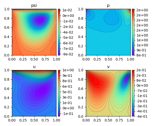
This module implements the Physics Informed Neural Network (PINN) model for the cavity flow governed by the equation of continuity and the steady Navier-Stokes equation in two dimensions. They are given by
u_x + v_y = 0,u*u_x + v*u_y + p_x/rho - nu*(u_xx + u_yy) = 0,u*v_x + v*v_y + p_y/rho - nu*(v_xx + v_yy) = 0,
where (u, v) is the flow velocity, p is the pressure, _x, _y indicate 1st derivatives d/dx, d/dy, _xx, _yy indicate 2nd derivatives d2/dx2, d2/dy2, rho is the density and nu is the viscosity. To fill the equation of continuity automatically, he sake of simplicity, we use the stream function psi given by (u = psi_y, v = -psi_x). For the cavity flow in the range x, y = 0 ~ 1, we give boundary conditions: u=1, v=0 at top boundary; u=0, v=0 at other boundaries, where Reynolds number Re=100 for rho=1 and nu=0.01. The PINN model predicts (psi, p) for the input (x, y).
The PINN is a deep learning approach to solve partial differential equations. Well-known finite difference, volume and element methods are formulated on discrete meshes to approximate derivatives. Meanwhile, the automatic differentiation using neural networks provides differential operations directly. The PINN is the automatic differentiation based solver and has an advantage of being meshless.
The effectiveness of PINNs is validated in the following works.
- M. Raissi, et al., Physics Informed Deep Learning (Part I): Data-driven Solutions of Nonlinear Partial Differential Equations, arXiv: 1711.10561 (2017).
- M. Raissi, et al., Physics Informed Deep Learning (Part II): Data-driven Discovery of Nonlinear Partial Differential Equations, arXiv: 1711.10566 (2017).
In addition, an effective convergent optimizer is required to solve the differential equations accurately using PINNs. The stochastic gradient dicent is generally used in deep learnigs, but it only depends on the primary gradient (Jacobian). In contrast, the quasi-Newton based approach such as the limited-memory Broyden-Fletcher-Goldfarb-Shanno method for bound constraints (L-BFGS-B) incorporates the quadratic gradient (Hessian), and gives a more accurate convergence.
Here we implement a PINN model with the L-BFGS-B optimization for the steady Navier-Stokes equation. In order to improve the convergence, we adopt swish activation in network.py and logcosh loss in optimizer.py .
Scripts is given as follows.
- lib : libraries to implement the PINN model for a projectile motion.
layer.py: computing derivatives as a custom layer.network.py: building a keras network model.optimizer.py: implementing the L-BFGS-B optimization.pinn.py: building a PINN model.tf_silent.py: suppressing tensorflow warnings
main.py: main routine to run and test the PINN solver.
You need Python 3.6 and the following packages.
| package | version (recommended) |
|---|---|
| matplotlib | 3.2.1 |
| numpy | 1.18.1 |
| scipy | 1.3.1 |
| tensorflow | 2.1.0 |
GPU acceleration is recommended in the following environments.
| package | version (recommended) |
|---|---|
| cuda | 10.1 |
| cudnn | 7.6.5 |
| tensorflow-gpu | 2.1.0 |
An example of PINN solver for the wave equation is implemented in main.py. The PINN is trained by the following procedure.
- Building the keras network model
The following table depicts layers in the default network.
from lib.network import Network
network = Network().build().
network.summary()
_________________________________________________________________ Layer (type) Output Shape Param # ================================================================= input_1 (InputLayer) [(None, 2)] 0 _________________________________________________________________ dense (Dense) (None, 32) 96 _________________________________________________________________ dense_1 (Dense) (None, 16) 528 _________________________________________________________________ dense_2 (Dense) (None, 16) 272 _________________________________________________________________ dense_3 (Dense) (None, 32) 544 _________________________________________________________________ dense_4 (Dense) (None, 2) 66 ================================================================= Total params: 1,506 Trainable params: 1,506 Non-trainable params: 0 _________________________________________________________________ - Building the PINN model.
from lib.pinn import PINN
pinn = PINN(network, rho=1, nu=0.01).build()
- Building training input.
# create training input
xy_eqn = np.random.rand(num_train_samples, 2)
xy_ub = np.random.rand(num_train_samples//2, 2)  # top-bottom boundaries
xy_ub[..., 1] = np.round(xy_ub[..., 1])          # y-position is 0 or 1
xy_lr = np.random.rand(num_train_samples//2, 2)  # left-right boundaries
xy_lr[..., 0] = np.round(xy_lr[..., 0])          # x-position is 0 or 1
xy_bnd = np.random.permutation(np.concatenate([xy_ub, xy_lr]))
x_train = [xy_eqn, xy_bnd]
- Building training output. We give the inlet velocity
u0=1.# create training output zeros = np.zeros((num_train_samples, 2)) uv_bnd = np.zeros((num_train_samples, 2)) uv_bnd[..., 0] = u0 * np.floor(xy_bnd[..., 1]) y_train = [zeros, zeros, uv_bnd]
- Optimizing the PINN model for the training data.
The progress is printed as follows. The optimization is terminated for loss ~ 1.8e-4.
from lib.optimizer import L_BFGS_B
lbfgs = L_BFGS_B(model=pinn, x_train=x_train, y_train=y_train)
lbfgs.fit()
Optimizer: L-BFGS-B (maxiter=20000)
9151/20000 [============>.................] - ETA: 17:56 - loss: 1.8428e-04
An example result (Reynolds number Re=100) is demonstrated below.
