Example Dataset location: https://drive.google.com/file/d/1sLc8Uk61W_4TTtmRk4x6_5cOiWq7IeOT/view?usp=sharing
Ole Peters
https://colab.research.google.com/github/ollimacp/spacial-boxcounting-cpu-gpu/blob/main/Spacial%20boxcount%20algorithm%20CPU%20and%20GPU.ipynb
This paper contains the postulation of a spacial boxcount algorithm, which characterizes any incoming 2D array spacially by indicators for topological complexity and spacial heterogenity at different scales. This characterization allows spacial similarity search or sorting capability, edge detection with userspecified scaling and statistical analysis of input datasets. The algorithm can handle any kind of data able to be represented in a 2 dimensional array. By training a convolutional neural network to mimic the cpu driven function, the process could speedup by a huge factor utilizing the parallel capabilities of a graphics card.
The daily advances in machine learning establish technological advances in almost any area of research. Convolutional neural networks gained a lot of traction, outperforming linear models and even recurrent models in timeseries forcasting. They often are used in object detection and are computationally intensive tasks.
Box counting like [1] is a method to analyze data by breaking the input array into boxes at different scales and counting every filled box indicating the spacial complexity for each scaling by the chosen the boxsize. An animation of this process is shown in figure 1.

Lacunarity is a mathematical discription for spacial heterogenity at a chosen scale [2]. With the boxcount and lacunarity, which depends on the boxsize, comparisons between different samples of the same data type can be made. By comparing these samples, similar structures can be found and sorted by spacial complexity and heterogenity. This enables characterization of continuously distributed data.

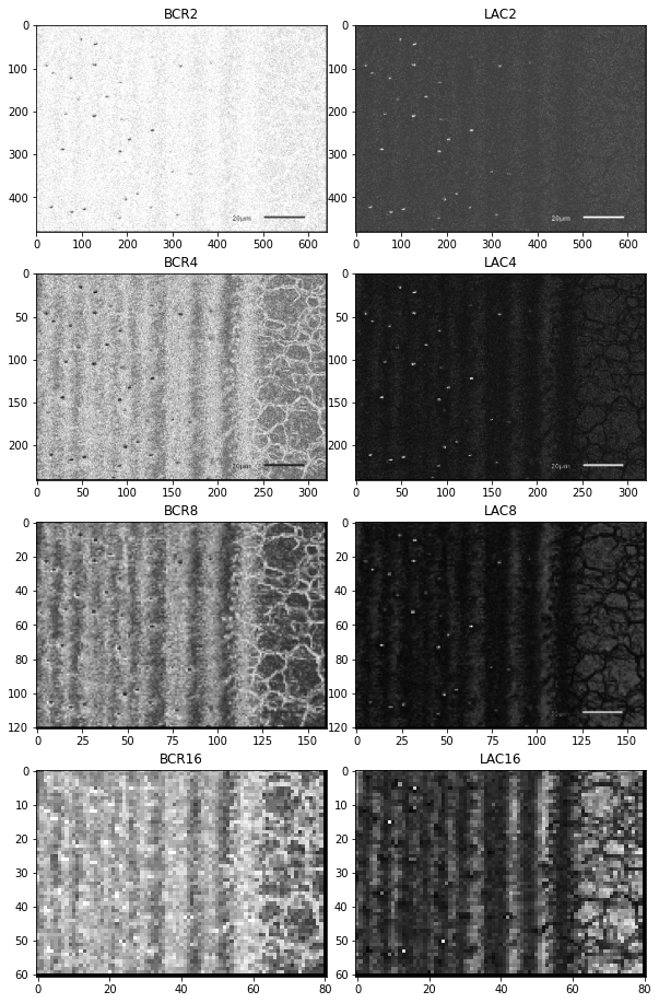
The spacial resolution of the boxcount algorithm can be achieved by chunking the picture into boxsize specified large areas, where within the boxcounting is executed resulting in a 2D array scaled inverse by the boxsize. These arrays represent the spacially distributed topological complexity and heterogenity at a chosen scale. The counted boxes reveal diffrent topological features and the lacunarity indicates defects in pattern respectively to their boxsizes. The boxsizes 2, 4, 8 and 16 were used, resulting in arrays with corresponding areas of 1/2, 1/4, 1/8, 1/16 of the original image size.
The dataset can be downloaded at: https://drive.google.com/file/d/1sLc8Uk61W_4TTtmRk4x6_5cOiWq7IeOT/view?usp=sharing
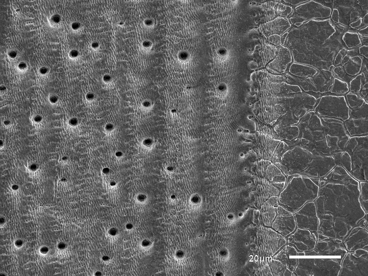
The example dataset consists of electron microscope images of femtosecond laser machined metal surfaces like the example shown in figure 3. These micro- and nanostructures are laser induced periodic surface structures, which are also known as LIPSS and can achieve drastic alterations on surface wettability. Also a few images of hydrophobic leaf surfaces are contained in the dataset.
Figure 3: Sample photo of a femtosecond laser machined metal surface with various surface features
In Figure 4 an output of the program has been generated, which results in pictures composed of boxcount ratios and lacunaritys at the chosen boxsize. Scale dependent features emerge at different boxsizes. The boxcount array indicates topological complexity, while contrast in the lacunarity array can distinguish spacial heterogen from homogen surface featuers.
Figure 4: Generated picture of resulting boxcount and lacunarity arrays with the boxsizes 2,4,8,16 reveal diffrent subpatterns derived from the surfacestructure.
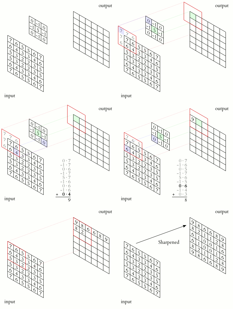
The concept of scanning arrays to count boxes or to perform a computation, like calculating the lacunarity, compared to the concept of convolutional neural networks with their kernel sized, stride moving convolution layers seem very similar. So a convolutional neural network could learn this task utilizing parallel processing power.
Figure 5: Animation of a convolution operation in a convolutional neural network.
Source: https://commons.wikimedia.org/wiki/File:2D_Convolution_Animation.gif


