This repository provides a starting point for the lab exercises of the course "Control and Perception in Networked and Autonomous Vehicles". You can find the course material on the CPM Lab website.
The code is organized as MATLAB packages in respective folders.
The folder +cmmn provides functionality which is shared between exercises.
Run the lab exercises in the CPM Lab.
The folder in which this code resides is expected to be software/high_level_controller/.
Control the vehicles as a platoon to drive along the predefined path, such that the leading vehicle follows a predefined reference velocity trajectory v_ref and other vehicles should maintain a constant distance d_ref to their front vehicles while considering the constraints in the Tab. 1.
Tab. 1: d_min refers to the minimal distance each vehicle should keep, v_min, v_max, a_min and a_max are minimal and maximal velocity, minimal and maximal acceleration, respectively.
More concretely, in this lab exercise five vehicles will be controlled to form a platoon, with vehicle IDs = [1,2,3,5,7], where the higher the vehicle's ID, the fronter the vehicle will be in the platoon. We notate the vehicle with ID n as vn, for example, vehicle with ID 7 will be notated as v7. In the platoon, the vehicle v5 follows v7, v3 follows v5, v2 follows v3, v1 follows v2. Thus, vehicle with ID 7 will be the leading vehicle of the platoon and vehicle with ID 1 will be the last vehicle.
The main task of this lab exercise is to implement different networked MPC strategies for networked and autonomous vehicles, especially the centralized MPC (CMPC) and distributed MPC (DMPC). Specifically, we will use priority based non-cooperative DMPC [1] for this lab exercise. At the end, the performance of these two kinds of networked MPC will be compared. At first, vehicle model is needed for MPC. Here we will use a linear discrete state-space model for MPC to predict vehicles' behavior; thus, the non-linear behavior of the vehicle will be approximated using linear state-space model. For model identification, the step response of the vehicle will be experimentally collected and analyzed using MATLAB's System Identification Toolbox (ssest). The identified system parameters are included in the system matrix A, input matrix B and output matrix C. This linear state-space model will be used throughout the total lab exercise. The implemented MPC strategies will be tested using simulation and experiment. The experiment will be carried out in Cyber-Physical Mobility Lab at the Chair of Embedded Software at RWTH Aachen University, where 20 networked model-scale (1:18) vehicles with maximum speed of 3.7 m/s can be used.
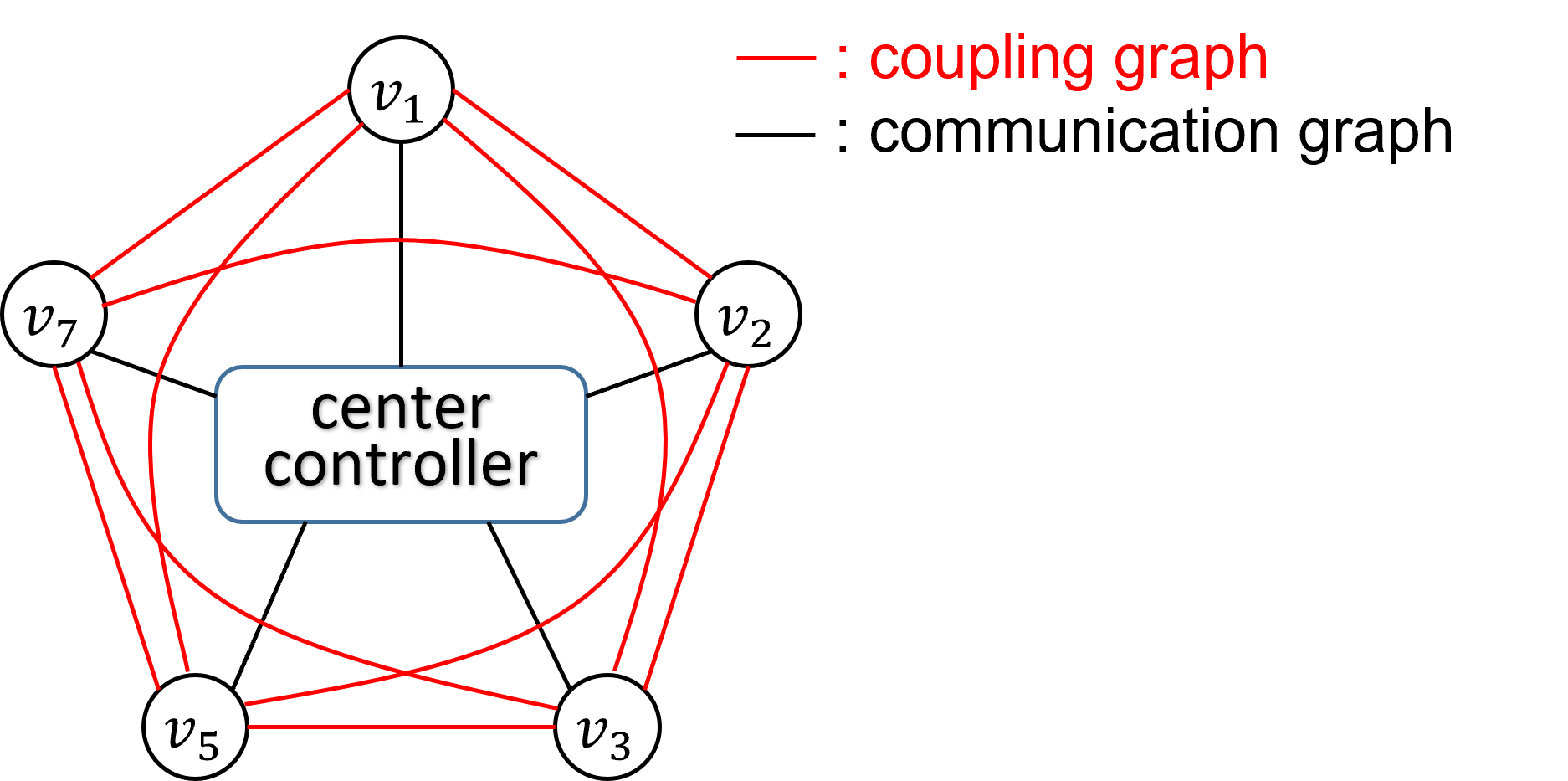
CMPC will be used in centralized platoon control. CMPC is characterized by the existence of a center controller that solves the optimization problem for the whole platoon and then send the optimized control input to each vehicle [1, p. 36]. The coupling and communication graph are shown in Fig. 1. Each vehicle communicates its states, reference trajectory and system parameters to the center controller. Therefore, the center controller has the complete information of the networked control system, which is able to form a single optimization problem. After solving the optimization problem, the center controller sends the optimal control input to each vehicle. The center controller plans for each vehicle under the consideration of all other vehicles' objective function and constraints, which leads to a fully connected coupling graph. The coupling and communication graphs are shown in Fig. 1.
Fig.1: Coupling and communication graphs of CMPC strategy, where, for example, v7 stands for vehicle with ID 7.
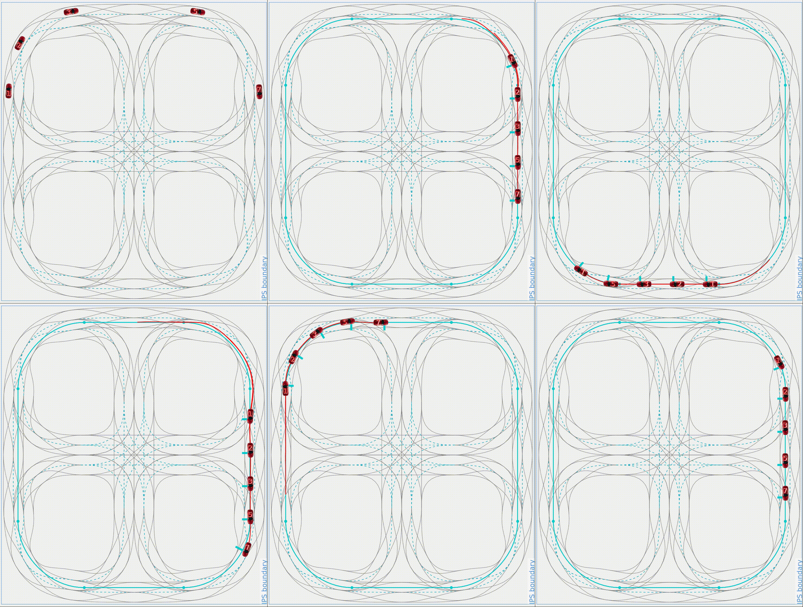
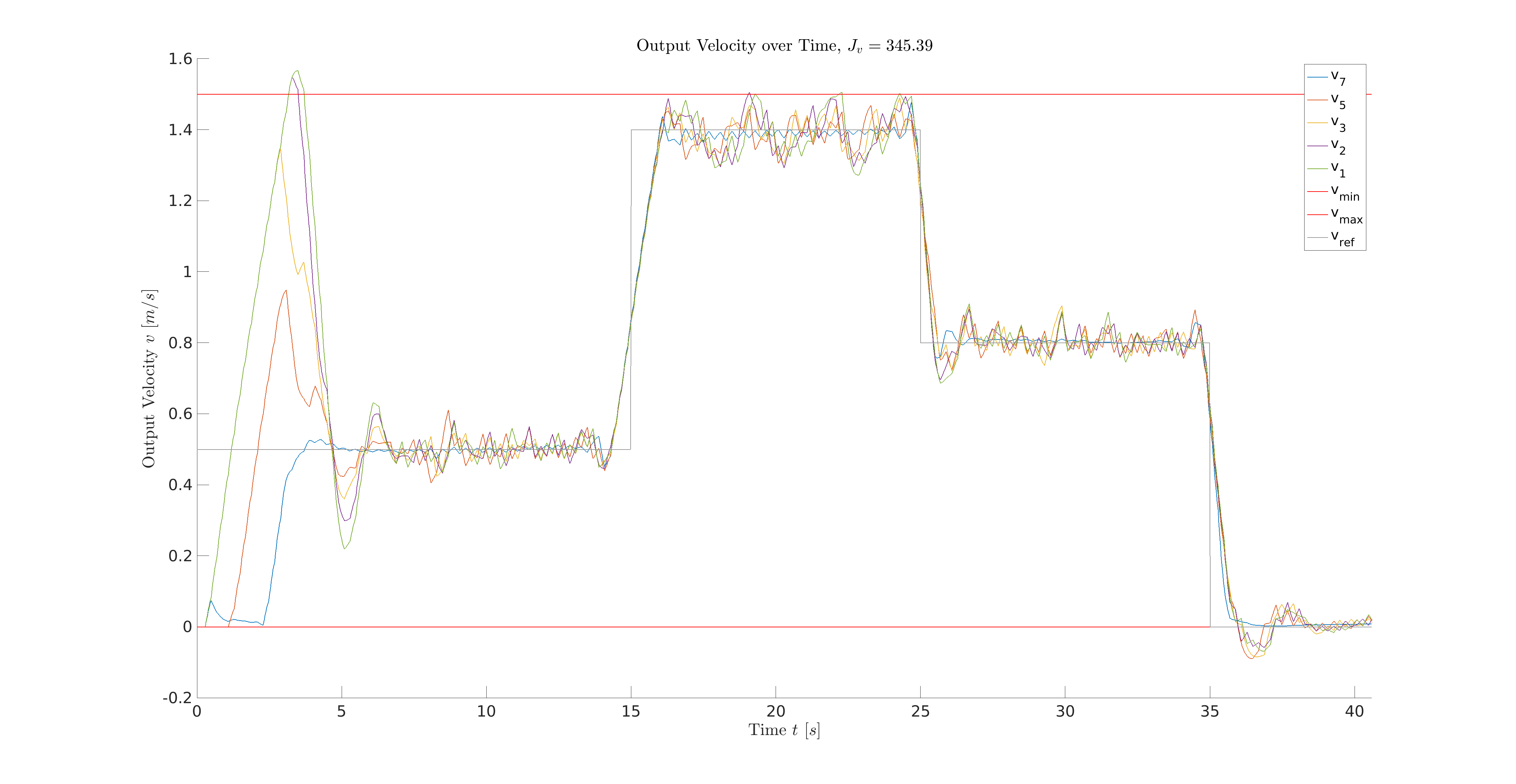
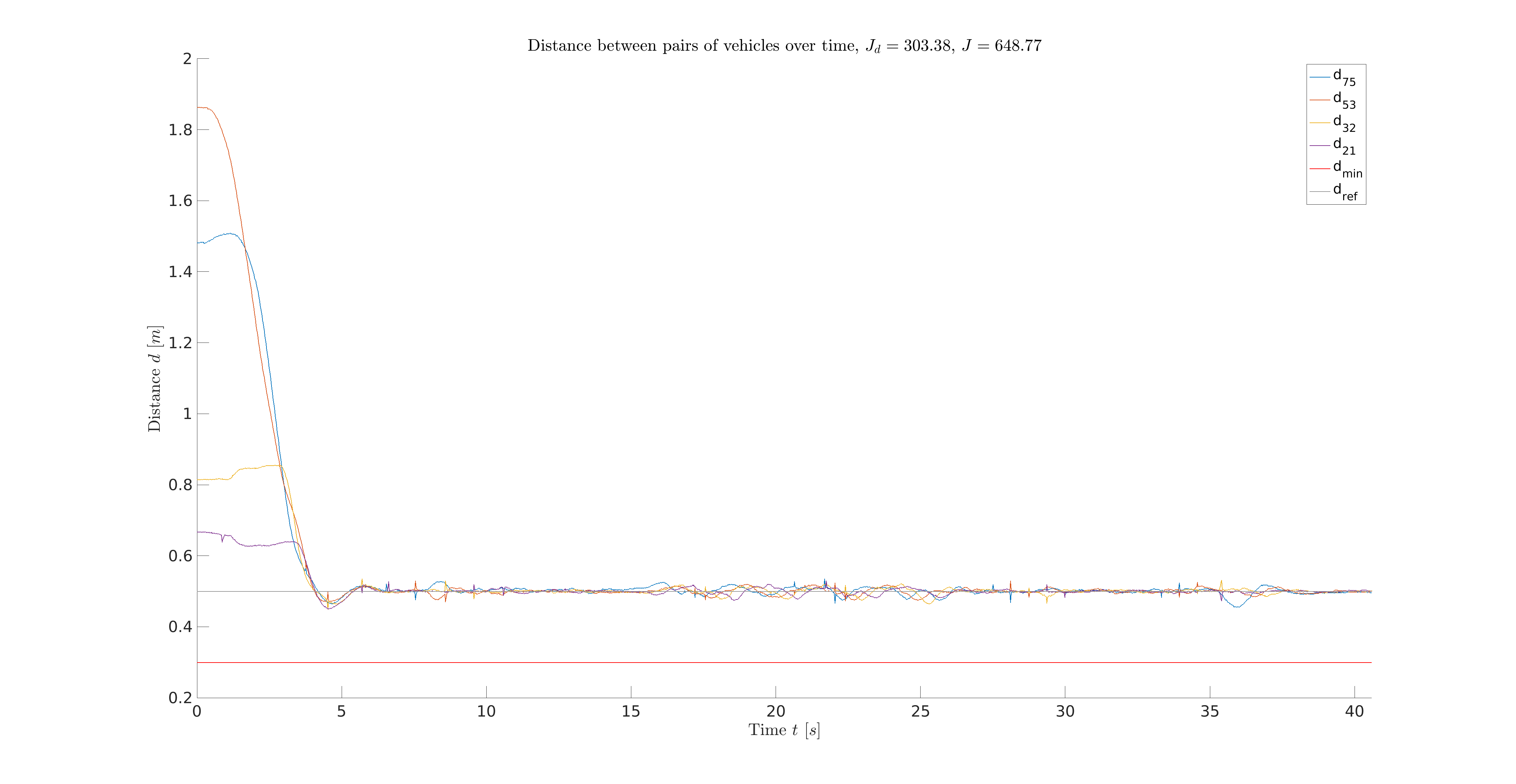
To form a centralized optimization problem, we firstly find a suitable state-space representation for the five vehicles. Specifically, the networked control system will be represented by a whole system matrix A_total, input matrix B_total and output matrix C_total. The output of the system is a five-dimensional vector. The first element is the velocity of the leading vehicle, the other four elements are the inter-vehicle distances. Thus, the optimization problem of the CMPC is to find an optimal input trajectory, which minimize the leading vehicle's velocity error and the inter-vehicle distance error under consideration of velocity and acceleration constraints. The optimization problem will be formed as a quadratic objective function with linear constraints such that it can be solved using MATLAB toolbox quadprog. The simulation recording is shown in Fig. 2 and the simulation results are shown in Fig. 3 and Fig. 4. The sum of squared error (SSE) of velocity tracking is shown in Fig. 3 with J_v = 345.4 and the SSE of distance tracking is shown in Fig. 4 with J_d = 303.4, which leads to the total SSE with J_total = J_v + J_d = 648.8. In the next section we could conclude that the SSE of both velocity and distance are far more less than those of the DMPC strategy. The drawbacks of the CMPC will also be discussed in the section III.
Fig. 2: Simulation recording using CMPC strategy. The number marked in the vehicle is its vehicle ID.
Fig. 3: Output velocity of each vehicle using CMPC strategy, where the upper and lower red horizontal lines represent the velocity input constraints, and the gray line represents the reference of the leading vehicle v1.
Fig. 4: Inter-vehicle distances using CMPC strategy, where the lower red horizontal line represents the minimal distance constraint and for example, v_75 stands for the distance between vehicle with ID 7 and ID 5.
DMPC will be used in distributed platoon control. There are two kinds of DMPC, cooperative DMPC and non-cooperative MPC. The main difference between them is that the former considers other vehicles' objective function while the latter not. In this lab exercise, non-cooperative DMPC will be used. To deal with the prediction inconsistence problem [1, p. 49] of the non-cooperative DMPC, in [1, p. 51] a novel non-cooperative DMPC is proposed, where each vehicle will be prioritized. The priority-based non-cooperative DMPC can reduce computation time as well using appropriate parallel computation. In our simple scenario, priority can be easily assigned: leading vehicle v7 has the highest priority, second vehicle v5 has the second highest priority, and so on. The coupling and communication graphs are shown in Fig. 5. The optimization problem is solved sequentially (see Tab. 2). In the for-loop, the leading vehicle's optimal input trajectory will be firstly calculated; then, the leading vehicle's predicted position under applying the optimal control input trajectory will be send to the second vehicle to calculate its reference position for the optimization problem. This will be repeated until every vehicle's optimal control input is calculated. Finally, the optimal control inputs will be applied to each vehicle. Though in each step N (number of vehicles) optimization problems are solved, the total computation time is still lower than CMPC because the number of decision variables and constraints of each optimization problem in DMPC is far less than the single optimization problem in CMPC, which makes the optimal solution easier to be found.
Fig. 5: Coupling and communication graphs of DMPC strategy, where v7 is the leading vehicle with the highest priority, v1 is the last vehicle of the platoon with the lowest priority. Both coupling and communication graphs are directed because only back vehicle should consider the front vehicle.
Tab. 2: Pseudocode of sequential computation
u_total = zeros(N,1) # initialize the control input for the whole platoon (totally N vehicles)

for i=1:N
  if i == 1 # leading vehicle
    [u_1,y_1] = optimizeMPC(v_ref) # solve the optimization problem with reference velocity trajectory as input
    u_total(1) = u_1(1)
  else # other vehicles
    [u_i,y_i] = optimizeMPC(y_(i-1)) # solve the optimization problem with position of the front vehicle as input
    u_total(i) = u_i(1)
  end
end

applyInput(u_total) # apply the optimal control input to the platoon
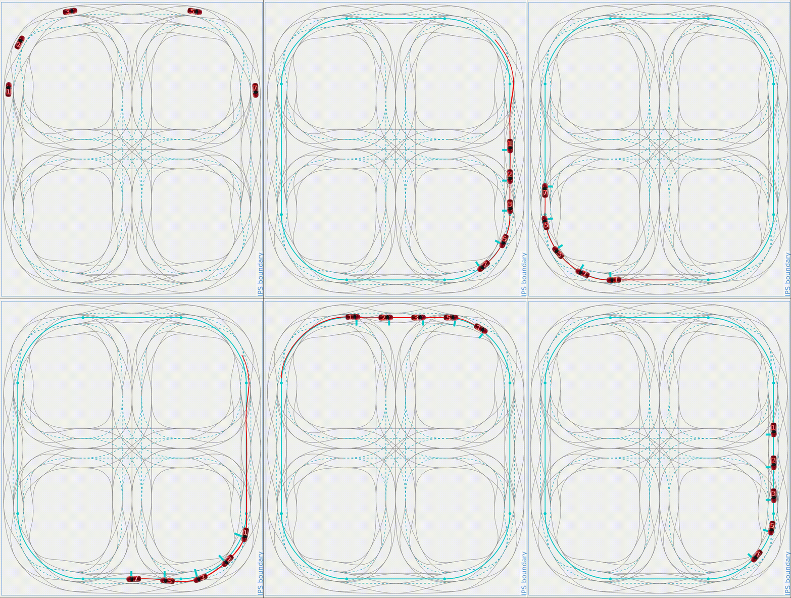
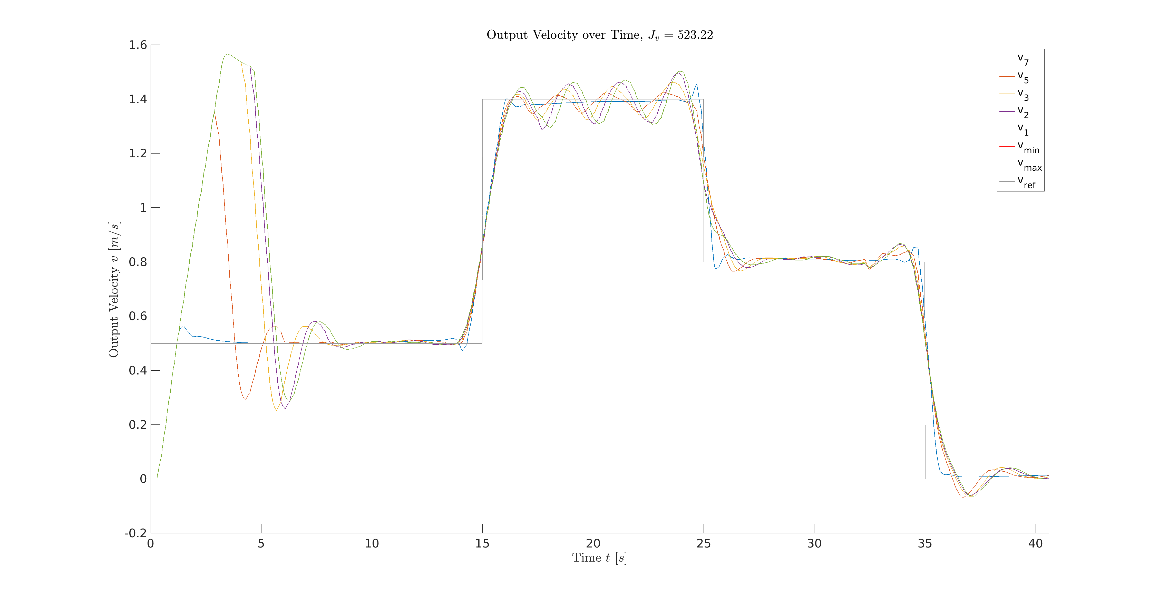
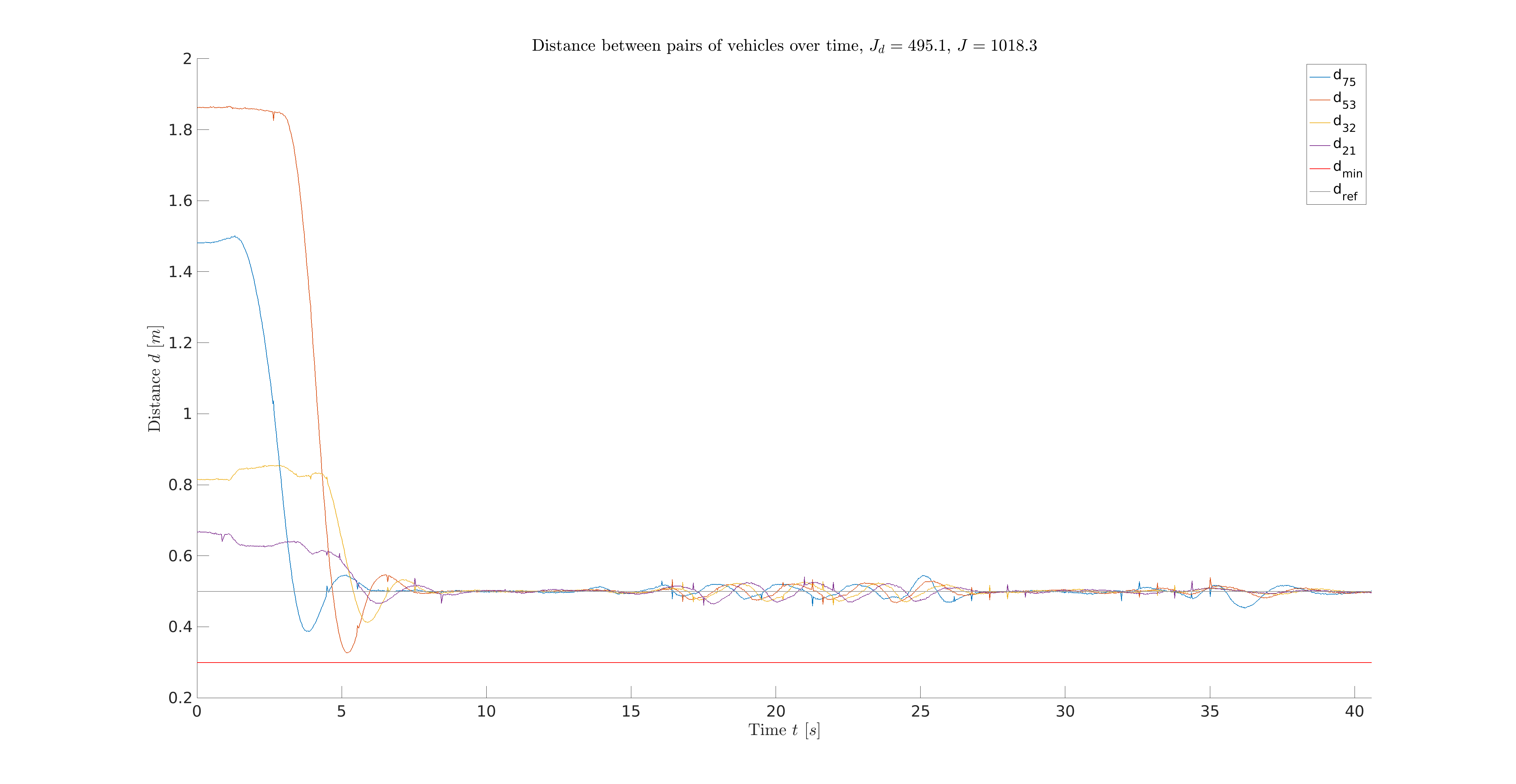
The simulation recording is shown in Fig. 6 and the simulation results are shown in Fig. 7 and Fig. 8. Fig. 7 demonstrates that the SSE of velocity tracking is J_v = 523.2 and the SSE of distance tracking is J_d = 495.1. The total SSE is therefore J_total = J_v + J_d = 1018.3.
Fig. 6: Simulation recording using DMPC strategy. The number marked in the vehicle is its vehicle ID.
Fig. 7: Output velocity of each vehicle using DMPC strategy, where the upper and lower red horizontal lines represent the input velocity constraints.
Fig. 8: Inter-vehicle distances using DMPC strategy, where the lower red horizontal line represents the minimal distance constraint and for example, v_75 stands for the distance between vehicle with ID 7 and ID 5.
In both CMPC and DMPC, the predictive horizon Hp is chosen to be 25 and control horizon Hu is chosen to be 12. Hp will be chosen such that the vehicle's dynamic will be covered by the whole predictive horizon and Hu should not exceed Hp. Normally, we can have a large control horizon, but considering the model used by MPC is an approximated linear model, we decide to choose Hu to be about a half of Hp. For comparison reason, the sample time for both CMPC and DMPC is 0.2 s. Note that a smaller sample time for DMPC can be chosen, for example 0.1 s, because later we can see that DMPC needs less computation time compared with CMPC.
The performances and computation time of CMPC and DMPC are compared in the Tab. 3. The performance of CMPC is obviously higher than DMPC. The SSE of the velocity tracking of CMPC is 345.5, which is about 50% lower than DMPC and the SSE of distance tracking of CMPC is almost 65% lower compared to DMPC. However, CMPC strategy needs 96 ms per step in average to solve the optimization problem, which is more than 30% compared to DMPC. The worst-case computation time of CMPC with 178 ms per step is 50% more than that of DMPC. This means a higher sample time is required when using CMPC strategy. For more vehicles, the computation time of CMPC grows exponentially, which makes it unsuitable for large-scale system. In addition, CMPC requires more complex communication system and has a single point of failure because it has only one controller, namely center controller [1, p. 38]. Compare to CMPC, DMPC is a good alternative to be used in the networked and autonomous vehicles, which has the advantage of low computation, though the performance is lower the CMPC. Its main advantage is the scalability. Using priority assignment to let optimization problems solved sequentially, the prediction inconsistency problem of traditional DMPC is addressed.
Tab. 3: Comparison of CMPC and DMPC strategies in the sense of computation time and performance for five vehicles.
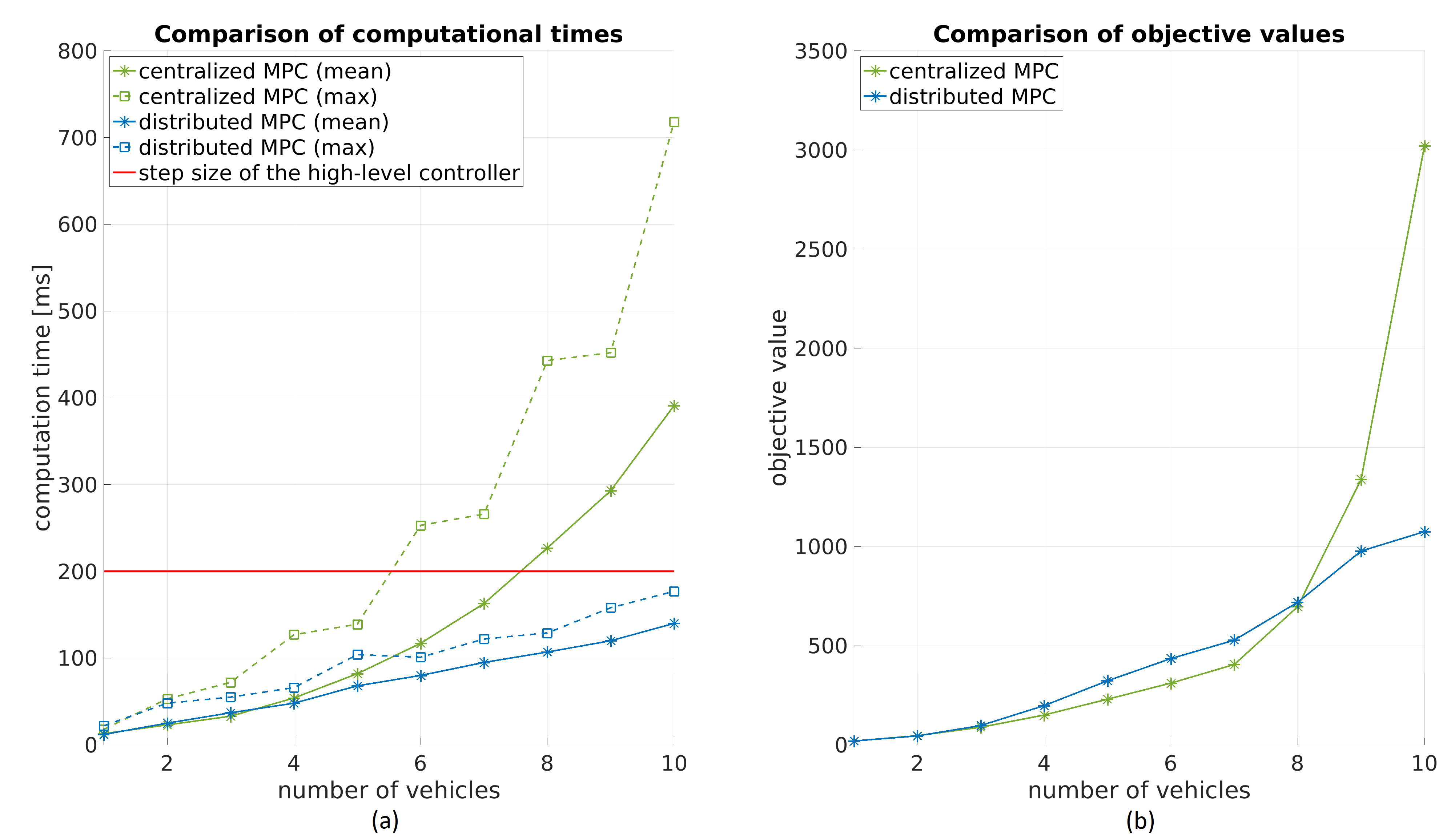
In our scenario, only five vehicles are considered. To get a more convincing comparison, we use the CMPC and DMPC to control from one to ten vehicles and plot the computation times and objective values. Fig. 9 (a) shows the maximal and mean computation time of the CMPC (green lines) and the DMPC (blue lines), where the step size of the high-level controller is shown by the horizontal red line (200 ms). The computation time of the CMPC grows exponentially with the number of vehicles, while that of the DMPC only increases roughly linear. This proves one of the previously mentioned drawbacks of the CMPC: poor scalability. Fig. 9 (b) compares the objective values of the CMPC and DMPC, which should be minimized in the optimization problem. The smaller the objective value, the lower velocity and distance tracking error and hence the higher the performance. From Fig. 9 (b) we can see that when the vehicle number is lower than 8, the performance of the CMPC is higher than the DMPC; but as the vehicle number grows to 8, the DMPC outperforms the CMPC. We can get the reason from Fig. 9 (a), where the mean computation time of the CMPC is larger than the step size of the high-level controller. This means that the CMPC is not real-time capable for vehicle number larger than 8, or in other words, the command inputs cannot be calculated in time when using CMPC. In such situation, the command inputs can, for example, remain the same as the previous time step, which is not good but better than zero. Even when the vehicle number grows to 6, the maximal computation time exceeds the step size. Therefore, the difference between the objective value of the CMPC and DMPC in Fig. 9 (b) is slowly decreasing after 6 vehicles.
Fig. 9: Comparison of CMPC and DMPC strategies in the sense of computation time and performance for different number of vehicles. Note that the objective value for five vehicles is not the same as it shows in Fig. 4 and Fig. 8 because we are using different vehicles (with IDs = [1,2,3,4,5] but not IDs = [1,2,3,5,7]). See Fig. 10 for the initial position of each vehicle. For n vehicles, the vehicles with IDs = [1,2,...,n] are used.
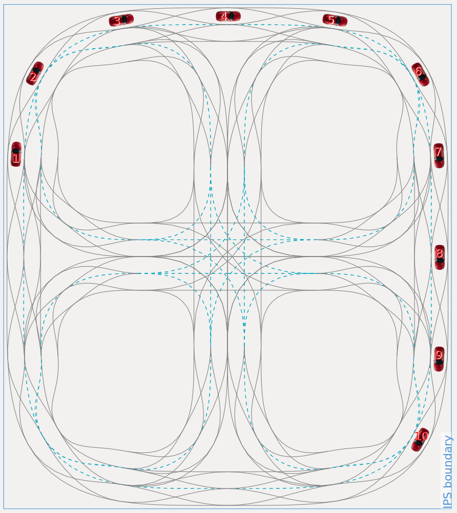
Fig. 10: Initial position of each vehicle.
[1] Alrifaee, Bassam. Networked model predictive control for vehicle collision avoidance. Diss. Dissertation, RWTH Aachen University, 2017, 2017.

