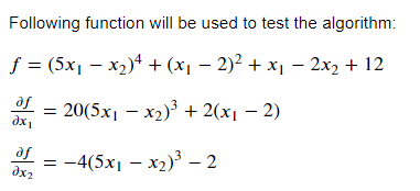
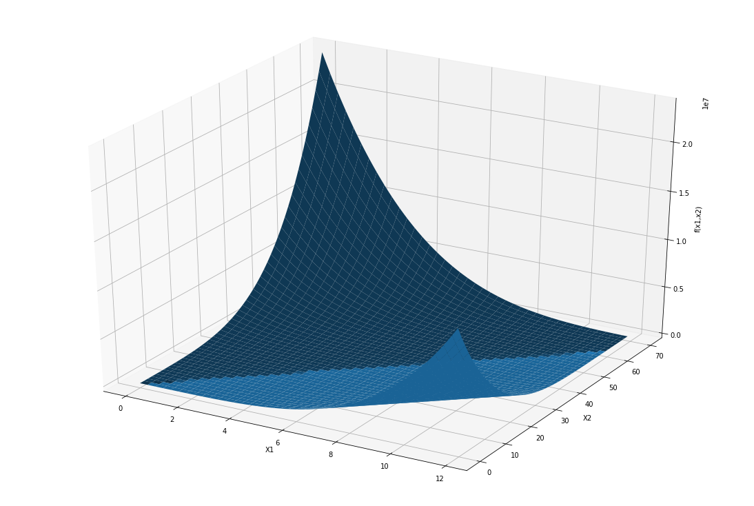
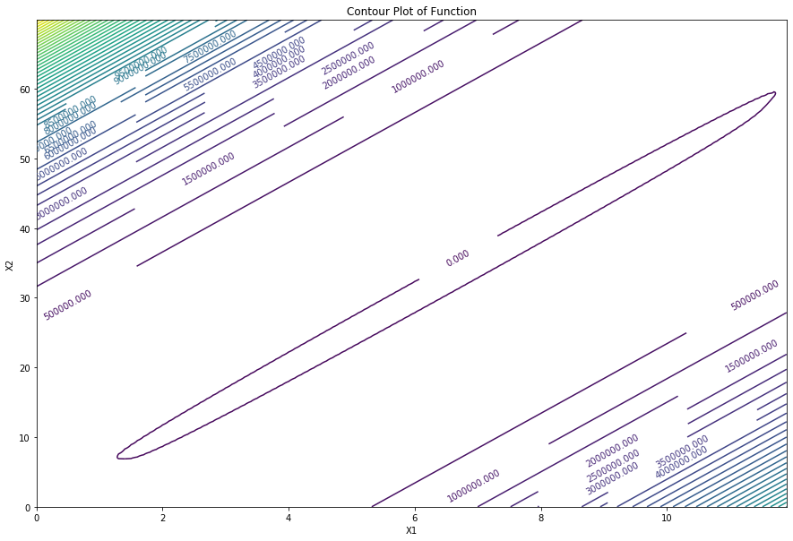
All imported packages are used to visualize the function and result of the algorithm.
import numpy as np
import matplotlib.pyplot as plt
from mpl_toolkits.mplot3d import Axes3D
from tabulate import tabulate
func = lambda x1,x2 :(5*x1-x2)**4 + (x1-2)**2 + x1 - 2*x2 + 12
funcx1 = lambda x1,x2 : 20*(5*x1-x2)**3 + 2*(x1-2)
funcx2 = lambda x1,x2 : -4*(5*x1-x2)**3 -2
# returns a new function where x2 is set to a constant c.
def set_x2_constant(c):
return (lambda x1 : (5*x1-c)**4 + (x1-2)**2 + x1 - 2*c + 12)
# returns a new function where x1 is set to a constant c.
def set_x1_constant(c):
return (lambda x2 : (5*c-x2)**4 + (c-2)**2 + c - 2*x2 + 12)# x1 and x2 are the intervals where function is plotted.
x1 = np.arange(0,12,0.1)
x2 = np.arange(0,70,0.1)
X1,X2 = np.meshgrid(x1,x2)
f = func(X1,X2)
fig = plt.figure()
ax = Axes3D(fig)
ax.plot_surface(X1,X2,f)
plt.xlabel('X1')
plt.ylabel('X2')
ax.set_zlabel('f(x1,x2)')
plt.gcf().set_size_inches(15, 10)
plt.show()fig,ax2 = plt.subplots()
cs = ax2.contour(X1,X2,f,50)
ax2.clabel(cs,inline=1,fontsize=10)
ax2.set_xlabel("X1")
ax2.set_ylabel("X2")
ax2.set_title('Contour Plot of Function')
plt.gcf().set_size_inches(15, 10)"""
GOLDEN SECTION METHOD
It finds the point where the f(x) is the minimum value of the convex function f.
f : function we want to find minimum value.
x_low : lower bound of the interval.
x_up : upper bound of the interval.
tol : tolerance is the stopping condition.
max_n: max number of iteration is also a stopping condition.
return: it returns the average of final interval's bounds which is
approximately equals to point where f(x) is minimum.
"""
def golden(f,x_low, x_up, tol, max_n):
iter_ctr = 0
while (x_up-x_low)>tol and iter_ctr<max_n:
x_n1 = x_up - 0.618*(x_up - x_low)
x_n2 = x_low + 0.618*(x_up - x_low)
if f(x_n1) <= f(x_n2):
x_up = x_n2
x_n2 = x_n1
x_n1 = x_up - 0.618*(x_up - x_low)
else:
x_low = x_n1
x_n1 = x_n2
x_n2 = x_low + 0.618*(x_up - x_low)
iter_ctr = iter_ctr + 1
return (x_n1 + x_n2)/2.0"""
CYCLIC COORDINATE SEARCH METHOD
It finds the point which is the global minimum of the two variable
function. => f(x1,x2)
f : function we want to find minimum value.
ip : initial points where algorithm starts.
return: it returns the points where f(x1,x2) is minimum and values while iterating.
"""
def cyclic_coordinate(f,ip):
x1,x2 = ip
results = [[0,x1,x2,f(x1,x2)]]
turn = 1
diff = 10**10
iter_ctr = 0
# epsilon could be changed to adjust the sensitivity of algorithm.
epsilon = 0.0001
while diff>epsilon:
func_x1 = set_x2_constant(x2)
func_x2 = set_x1_constant(x1)
if (turn == 1):
new_x1 = golden(func_x1,x1-5000,x1+5000,0.0001,100)
diff = abs(f(x1,x2)-f(new_x1,x2))
x1 = new_x1
turn = 2
else:
new_x2 = golden(func_x2,x2-5000,x2+5000,0.0001,100)
diff = abs(f(x1,x2)-f(x1,new_x2))
x2 = new_x2
turn = 1
iter_ctr += 1
results.append([iter_ctr,x1,x2,f(x1,x2)])
return results# this is the point where algorithm starts. points with high function value could cause
# overflow since the chosen function increases rapidly.
initial_point = [1,60]
ccs = cyclic_coordinate(func,initial_point)
print(tabulate(ccs[:10]+ccs[-10:],headers=['Iteration','x1','x2','f(x1,x2)'])) Iteration x1 x2 f(x1,x2)
----------- -------- ------- -------------
0 1 60 9.15052e+06
1 11.798 60 0.839408
2 11.798 59.7838 0.628533
3 11.7551 59.7838 0.383139
4 11.7551 59.5691 0.175354
5 11.7124 59.5691 -0.0662981
6 11.7124 59.3559 -0.271019
7 11.6701 59.3559 -0.50907
8 11.6701 59.1439 -0.711115
9 11.6279 59.1439 -0.945628
812 6.60187 33.8031 -27.4302
813 6.60083 33.8031 -27.4303
814 6.60083 33.7979 -27.4304
815 6.59979 33.7979 -27.4305
816 6.59979 33.7927 -27.4306
817 6.59874 33.7927 -27.4307
818 6.59874 33.7874 -27.4308
819 6.5977 33.7874 -27.4309
820 6.5977 33.7822 -27.431
821 6.5967 33.7822 -27.4311
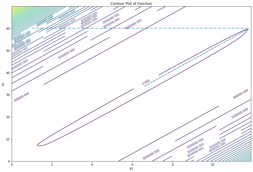
ccs=np.array(ccs)
fig,ax2 = plt.subplots()
cs = ax2.contour(X1,X2,f,50)
ax2.clabel(cs,inline=1,fontsize=10)
ax2.set_xlabel("X1")
ax2.set_ylabel("X2")
ax2.set_title('Contour Plot of Function')
plt.plot(ccs[:,1],ccs[:,2],'-.')
plt.gcf().set_size_inches(15, 10)
In this image every dot represent one iteration of cyclic cordinate search algorithm. Basically algorithm find a direction where function's value gets smaller and moves on that direction until function's value do not get smaller. Then it finds a new direction to move. On the next cells algorithm will be tried with a simpler function.


