Used different Transformer based and LSTM based models for forecasting rainfall in different areas of Mumbai. Employed different smart training techniques to improve correlation with the true time-series.
The data that was available to me had Rainfall, windspeed, GFS forecast and Co-ordinates of different AWS stations in Mumbai. The first data processing task was to combine all of these into a single csv file. The data was collected by 37 stations all over Mumbai at time-intervals of 15 minutes in the years 2015-22. Rainfall and Windspeed data was combined as it is after basic preprocessing like removal of nan values. GFS predictions had to be shifted left in timeline by 15 minutes so that they can also be used as parameters to our model. So the final csv file that was generated had 93695 rows, where each row had (37 + 37 + 37 = 111) features. You can find the code which does all of the above things here
The main aim of this project was to predict the rainfall in different areas of Mumbai for the next 3 hours at a lead-time of 15 minutes when all the 111 features for the past 3 hours were provided at an interval of 15 minutes. So, the shape of the input to our model is (12, 111) while the output dimension is (12, 1) for each of the 37 stations.
The above dataset was now broken into 2 DataFrames, 1 each for training and testing with a training spilt of 0.9. It means that the shape of the DataFrame used for generating the training data is (84325, 111) while that used for generating the test data is (9370, 111). Now, the above 2 dataframes were normalized using min-max Normalization where the min and max values for each of the 111 features were computed using only the Train DataFrame. Those same values were later used to Normalize the test DataFrame before feeding to the model and Re-Normalizing the outputs back to their original values after the model evaluation.
Now, we have the normalized data. Then I made the 2, 3 Dimentional Arrays for x_train and x_test each of which had the no of samples as the 1st dimension, lead-time as the 2nd dimension and features as the 3rd dimension. I also made y_train and y_test each of which is a 2D array for each of the stations. no of samples is the 1st dimension and lead-time as the 2nd dimension. All of these arrays were converted into tensors and split into different batches after shuffling to ensure that the model learns the true characteristics of predicting Rainfall rather than just extrapolating the previous values.
I used the following 3 model architectures for predicting the future rainfall. Two of these models are based on LSTM architecture while one of these uses the Transformer architecture.
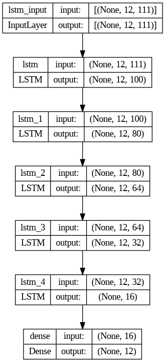
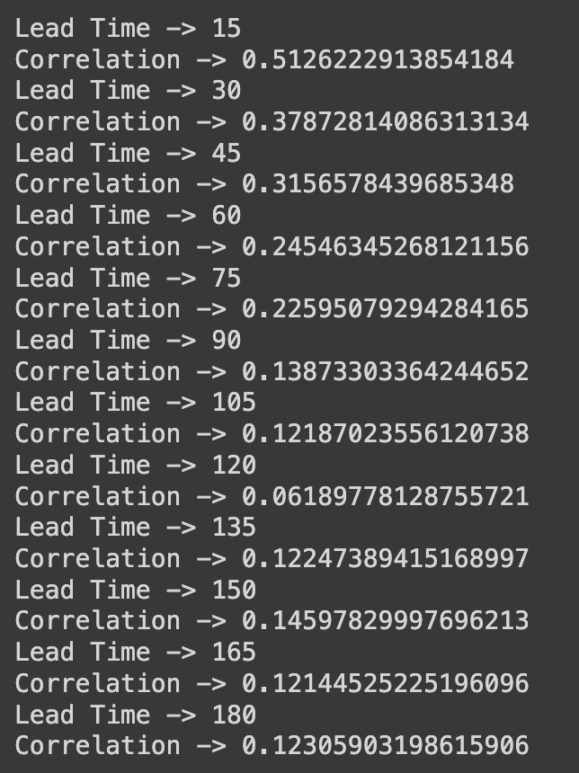
This model was programmed in TensorFlow using the Sequential API. The model had a couple of layers with gradually reducing number of units for smooth flow of only the relevant information. This gave the best correlation of 51 % with the target output time series. The Source code for this model can be found here. The trained model weights for Andheri can be found here. The Model Architecture, correlation values and time series plot for one of the stations (Andheri) is given below ->
 |
 |
|---|---|
| Model Architecture | Correlation values with original time series |
 |
|---|
| plot of time series of Andheri prediction |
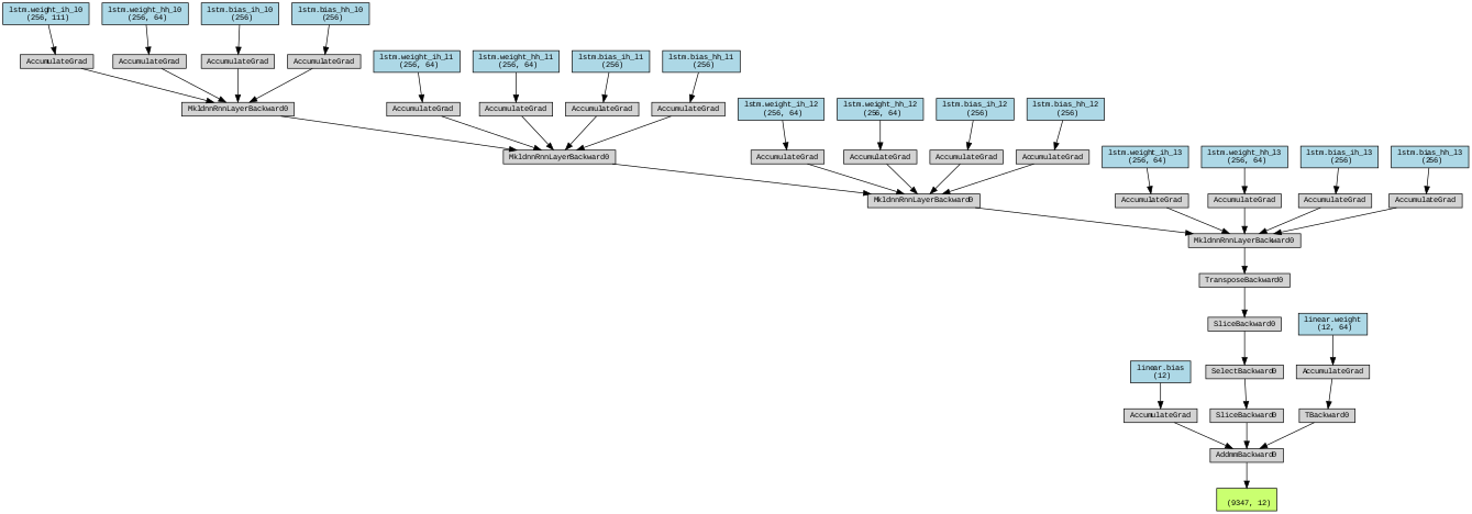
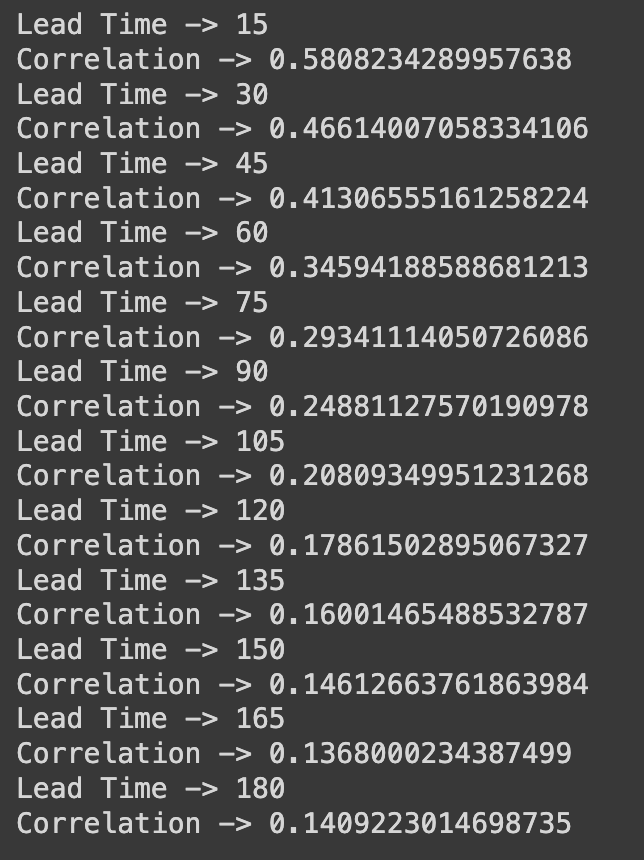
This model was programmed in PyTorch. This model has 4 identical layers with a predefined dimention for the hidden-states. This model gave a best correlation of around 58 % with the target time series. The Source code for this model can be found here. The trained model weights for Andheri can be found here. The Model Architecture, correlation values and time series plot for one of the stations (Andheri) is given below ->
 |
 |
|---|---|
| Model Architecture | Correlation values with original time series |
 |
|---|
| plot of time series of Andheri prediction |
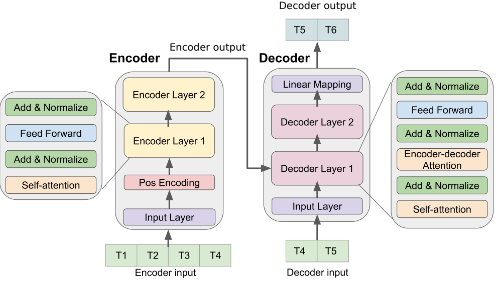
This model makes use of the pre-defined transformer model in PyTorch. I have also additionally included positional encoding block which allows the transformer model to learn the relative positional significance of different lead-times in the input while predicting the future rainfall values. The model has 2 inputs, 1 each for the Encoder and Decoder of the Transformer. So for this model we need 3 arrays instead of the 2 that we used in the earlier 2 models. There should be non-zero overlap between both input to encoder-input to decoder and input to decoder-output of the model. So, encoder input is of 24 timesteps, decoder input as well as the transformer output is of 16 timesteps. The details of the model architecture as well as the input and output dimensions of the model can be understood by looking at the source code here. The model architecture is as follows ->
