+ Update V2.0.1 (June 2017):
+ Updated documentation to include Visual Object Tagging Tool as an annotation option.
+ Update v2 (June 2017):
+ Updated code to be compatible with the CNTK 2.0.0 release.
+ Update v1 (Feb 2017):
+ This tutorial was updated to use CNTK's python wrappers. Now all processing happens in-memory during scoring. See script 6_runSingleImage for an example. Furthermore, we switched to a much more accurate and faster implementation of Selective Search.
+ Note that, at the time of writing, CNTK does not support Python 2. If you need Python 2 then please refer to the [previous version](https://github.com/Azure/ObjectDetectionUsingCntk/tree/7edd3276a189bad862dc54e9f73b7cfcec5ae562) of this tutorial.Object Detection is one of the main problems in Computer Vision. Traditionally, this required expert knowledge to identify and implement so called “features” that highlight the position of objects in the image. Starting in 2012 with the famous AlexNet paper, Deep Neural Networks are used to automatically find these features. This lead to a huge improvement in the field for a large range of problems.
This tutorial uses Microsoft Cognitive Toolkit's (CNTK) fast R-CNN implementation (see the Fast R-CNN section for a description) which was shown to produce state-of-the-art results for Pascal VOC, one of the main object detection challenges in the field.
The goal of this tutorial is to show how to train and test your own Deep Learning object detection model using Microsoft Cognitive Toolkit (CNTK). Example data and annotations are provided, but the reader can also bring their own images and train their own, unique, object detector.
The tutorial is split into four parts:
- Part 1 shows how to train an object detection model for the example data without retraining the provided Neural Network, but instead training an external classifier on its output. This approach works particularly well with small datasets, and does not require expertise with deep learning.
- Part 2 extends this approach to refine the Neural Network directly without the need for an external classifier.
- Part 3 illustrates how to annotate your own images and use these to train an object detection model for your specific use case.
- Part 4 covers how to reproduce published results on the Pascal VOC dataset.
Previous expertise with Machine Learning while not required to complete this tutorial, however is very helpful to understand the underlying principles. More information on the topic can also be found at CNTK's Fast-RCNN page.
This tutorial was tested using CNTK v2.0.0, and assumes that CNTK was installed with the (default) Anaconda Python interpreter. Note that the code will only run on v2.0 due to breaking changes in other versions.
CNTK can be easily installed by following the instructions on the script-driven installation page. This will also automatically add an Anaconda Python distribution. At the time of writing, the default python version is 3.5.
A dedicated GPU is not required, but recommended for retraining of the Neural Network (part 2). If you lack a strong GPU, don't want to install CNTK yourself, or want to train a model using multiple GPUs, then consider using Azure's Data Science Virtual Machine. See the Cortana Intelligence Gallery for a 1-click deployment solution.
Several Python packages are required to execute the python scripts. These libraries can be installed easily using provided python wheels by opening a command prompt and running:
c:/local/CNTK-2-0/cntk/Scripts/cntkpy35.bat
cd resources/python35_64bit_requirements/
pip.exe install -r requirements.txt
In the code snippet above, we assumed that the CNTK root directory is C:/local/CNTK-2-0/. The python wheels were originally downloaded from this page.
Finally, the file AlexNet.model is too big to be hosted in Github and hence needs to be downloaded manually from here and placed into the subfolder /resources/cntk/AlexNet.model.
| Folder | Description |
|---|---|
| / | Root directory |
| /data/ | Directory containing images for different object recognition projects |
| /data/grocery/ | Example data for grocery item detection in refrigerators |
| /data/grocery/positives/ | Images and annotations to train the model |
| /data/grocery/negatives/ | Images used as negatives during model training |
| /data/grocery/testImages/ | Test images used to evaluate model accuracy |
| /doc/ | Resources such as images for this readme page |
| /fastRCNN/ | Slightly modified code used in R-CNN publications |
| /resources/ | All provided resources are in here |
| /resources/cntk/ | CNTK configuration file and pre-trained AlexNet model |
| /resources/python35_64_bit_requirements/ | Python wheels and requirements file for 64bit Python version 3.5 |
All scripts used in this tutorial are located in the root folder.
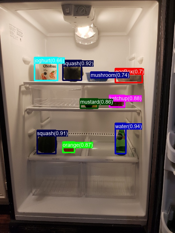
In the first part of this tutorial we will train a classifier which uses, but does not modify, a pre-trained deep neural network. See the Fast R-CNN section for details of the employed approaches. As example data 25 images of grocery items inside refrigerators are provided, split into 20 images for training and the remaining 5 images are used as test set. The training images contain in total 180 annotated objects, these are:
Egg box, joghurt, ketchup, mushroom, mustard, orange, squash, and water.
Note that 20 training images is a very low number and too little train a high-accuracy detector. Nevertheless, even this small dataset is sufficient to return plausible detections as can be seen in step 5.
Every step has to be executed in order, and we recommend after each step to inspect which files are written, where they are written to, and what the content of these files is (mostly the content is written as text file).
Script: 1_computeRois.py
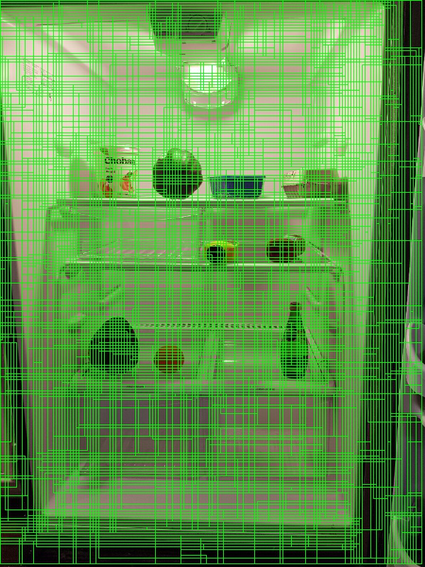
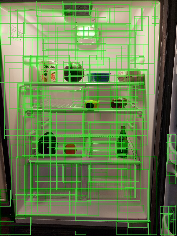
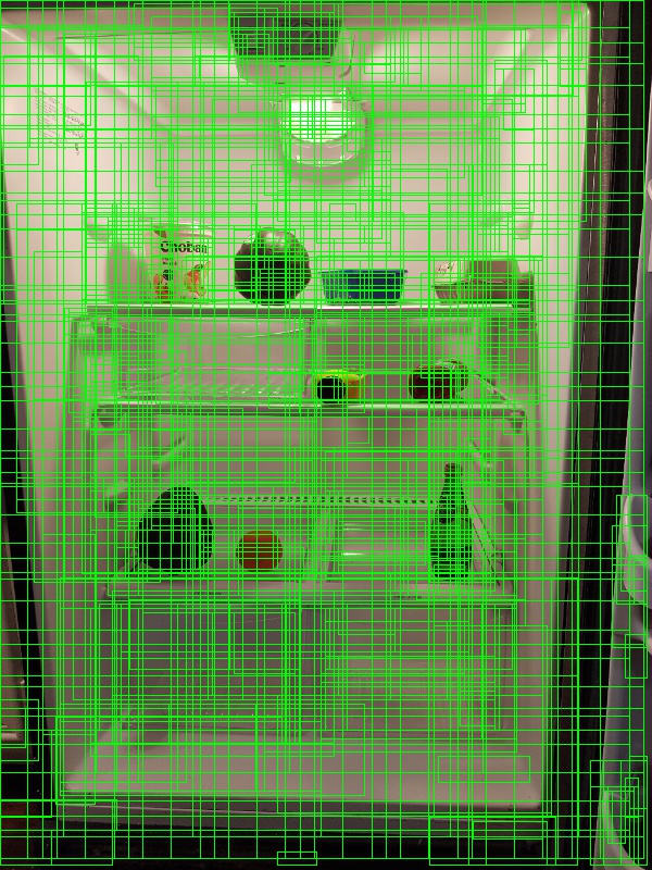
Region-of-interests (ROIs) are computed for each image independently using a 3-step approach: First, Selective Search is used to generate hundreds of ROIs per Image. These ROIs often fit tightly around some objects but miss other objects in the image (see Selective Search section). Many of the ROIs are bigger, smaller, etc. than the typical grocery item in our dataset. Hence in a second step these ROIs, as well as ROIs which are too similar, are discarded. Finally, to complement the detected ROIs from Selective Search, ROIs that uniform cover the image are added at different scales and aspect ratios.
The final ROIs are written for each image separately to the files [imageName].roi.txt in the proc/grocery/rois/ folder.
For the grocery dataset, selective search typically generates around 1000 ROIs per image, plus on average another 2000 ROIs sampled uniformly from the image. A high number of ROIs typically leads to better object detection performance, at the expense however of longer running time. Hence the parameter cntk_nrRois can be used to only keep a subset of the ROIs (e.g. if cntk_nrRois = 2000 then typically all ROIs from selective search are preserved, plus the 1000 largest ROIs generated using uniform sampling).
The goodness of these ROIs can be measured by counting how many of the ground truth annotated objects in the image are covered by at least one ROI, where "covered" is defined as having an overlap greater than a given threshold. Script B1_evaluateRois.py outputs these counts at different threshold values. For example for a threshold of 0.5 and 2000 ROIs, the recall is around 98%, while with 200 ROIs the recall is around 85%. It is important that the recall at a threshold of 0.5 is close to 100%, since even a perfect classifier cannot find an object in the image if it is not covered by at least one ROI.
ROIs computed using Selective Search (left); ROIs from the image above after discarding ROIs that are too small, too big, etc. (middle); Final set of ROIs after adding ROIs that uniformly cover the image (right).
Script: 2_cntkGenerateInputs.py
Each ROI generated in the last step has to run through the CNTK model to compute its 4,096 float Deep Neural Network representation (see the Fast R-CNN section). This requires three CNTK-specific input files to be generated for the training and the test set:
- {train,test}.txt: each row contains the path to an image.
- {train,test}.rois.txt: each row contains all ROIs for an image in relative (x,y,w,h) co-ordinates.
- {train,test}.roilabels.txt: each row contains the labels for the ROIs in one-hot-encoding.
An in-depth understanding of how these files are structured is not necessary to understand this tutorial. However, two points are worth pointing out:
- CNTK’s fast R-CNN implementation requires all images to be of the same size. For this reason, all images are first scaled and then centered and zero-padded (i.e. columns of gray-colored pixels are added to the left and right of the image, or respectively rows at the top and bottom). Note that the scaling preserves the original aspect ratio. For our experiments we use input width and height of 1000 x 1000 pixels to the Neural Network.
Interestingly, upscaling an image can significantly improve accuracy if the objects to be detected are small (this is due to objects in ImageNet typically having a width and height of 100-200 pixels). - CNTK expects each image to have the same number of ROIs (for our experiments we use 2000). Hence, if the computation in step 1 returned more ROIs, then only the first 2000 are used. Likewise, if less ROIs were found, then the remaining spots are filled using ROIs with co-ordinates of (0,0,0,0). These “zero-padded” ROIs are only used during CNTK execution and have no influence on the training / test performance.
This step writes the above mentioned files to the directory proc/grocery/cntkFiles/. For debugging, the script B2_cntkVisualizeInputs.py can be used to visualize the content of these files (e.g. the Figure at the end of step 4 was generated using this script).
Script: 3_runCntk.py
We can now run the CNTK training which takes as input the co-ordinates and labels files from the last step and writes the 4096 float embedding for each ROI and for each image to proc/grocery/cntkFiles/{train,test}_svm_parsed/[imageName].dat.npz. This will take a few minutes, and will automatically run on GPU if detected.
Note: Look for the line "Using GPU for training." in the console output to make sure the training runs on GPU and not CPU (which would be too slow). Note that a previous CNTK run might still be open and holding a block on the GPU.
Script: 4_trainSvm.py
We now train the classifier which given an ROI as input, assigns it to one of the grocery items or to a “background” class.
We use a slightly modified version of the published R-CNN code to train a linear SVM classifier. The main change is to load the 4096 floats ROI embedding from disk rather than to run the network on-the-fly. An in-depth explanation of the training procedure can be found in the R-CNN paper. For the purpose of this tutorial we consider the training script a black box, which uses the training ROIs as input (or to be precise the 4096 floats representations), and outputs N+1 linear classifiers, one for each class, plus one for the background.
The training starts by loading all positive ROIs into memory. Positive here corresponds to each ROI that has a significant overlap with a ground truth annotated object. Negatives are then iteratively added using hard negative mining, and the SVM is retrained. A list and short description of the parameters that govern the SVM training can be found in the script PARAMETERS.py.
The learned linear classifiers for each class, i.e. a weight vector of dimension 4096 floats plus a float that represents the bias term, are then written to the folder proc/grocery/trainedSVMs/.
Scripts: 5_evaluateResults.py and 5_visualizeResults.py
Once training succeeded, the model can be used to find objects in images. For this, every ROI in an image is classified and assigned a confidence to be orange, ketchup, ... and background. The class with highest confidence is then selected (most often “background”) and optionally a threshold applied to reject detections with low confidence.
The accuracy of the classifier can be measured using the script 5_evaluateResults.py. This outputs the mean Average Precision (mAP; see the Mean Average Precision section) for either the training or the test set. Keep in mind that the test set only contains 5 images and hence these numbers need to be taken with a grain of salt. Due to randomization effects one might get very different results when running the script.
Results using 200 ROIs (this number is too low to get good accuracy but for demo purposes allows for fast training and scoring):
| Dataset | AP(orange) | AP(eggBox) | AP(joghurt) | AP(ketchup) | mAP | |
|---|---|---|---|---|---|---|
| Test Set | 0.45 | 1.00 | 0.82 | 0.76 | 0.63 |
Results using 2000 ROIs:
| Dataset | AP(orange) | AP(eggBox) | AP(joghurt) | AP(ketchup) | mAP | |
|---|---|---|---|---|---|---|
| Test Set | 0.32 | 0.48 | 0.82 | 0.82 | 0.65 |
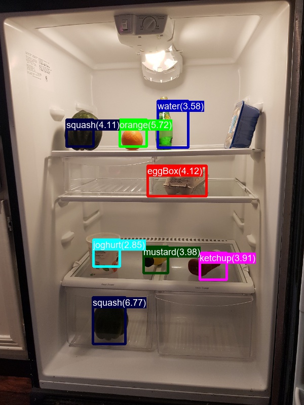
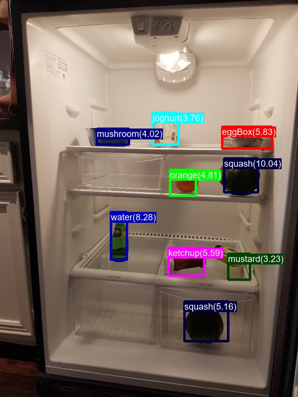
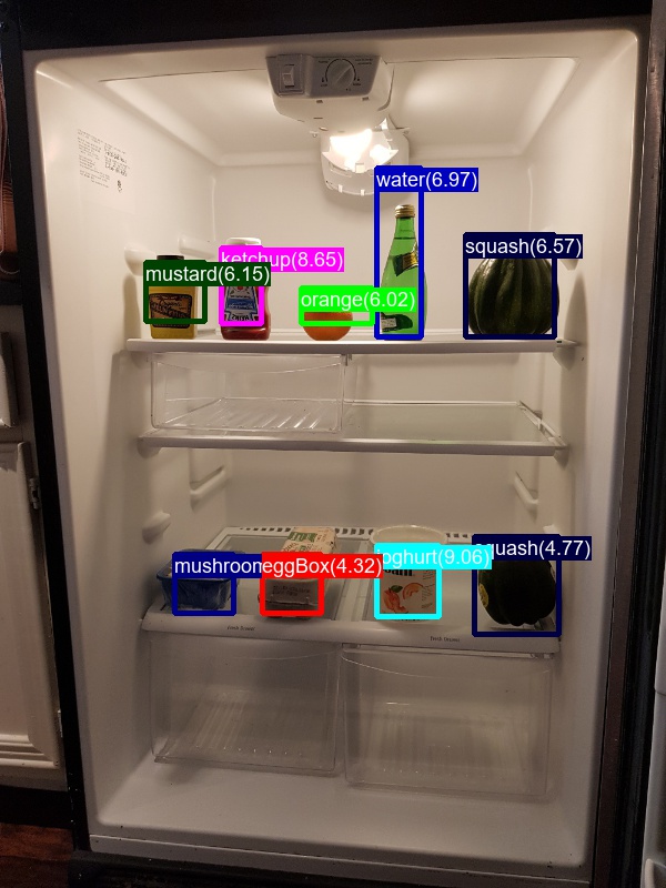
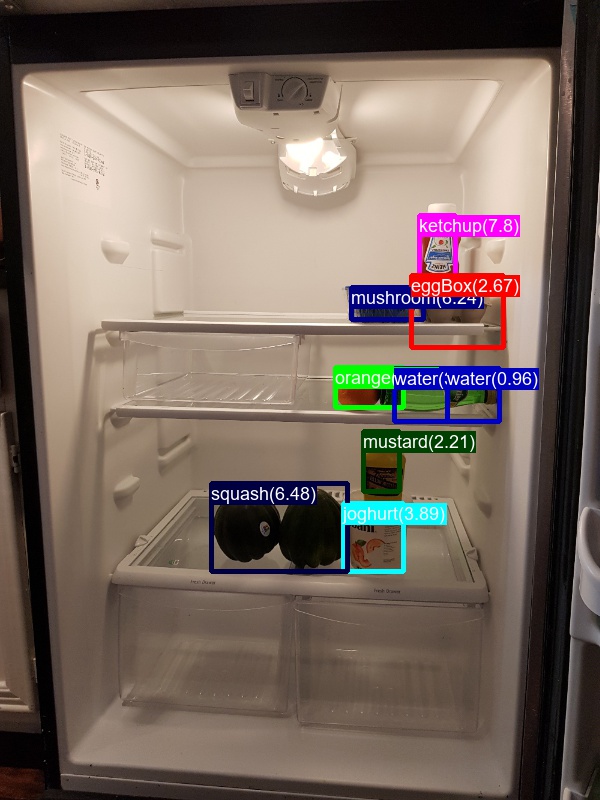
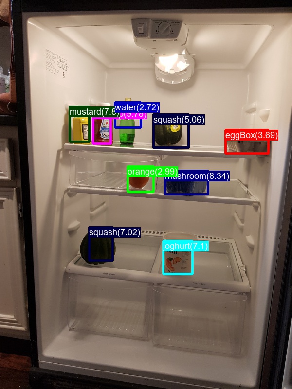
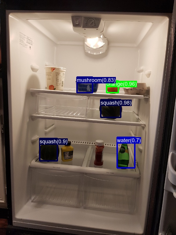
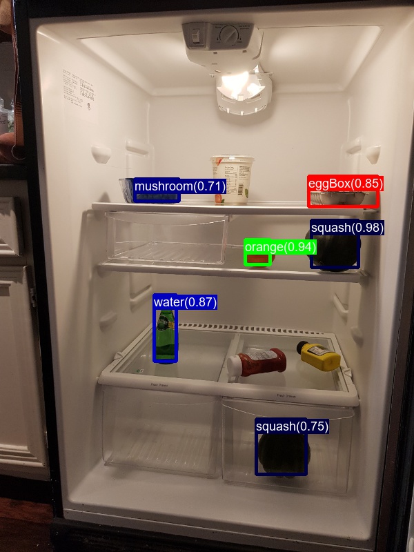
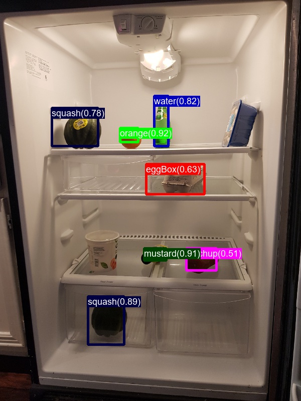
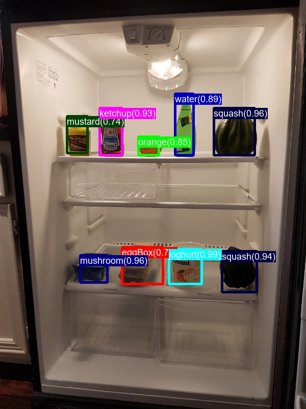
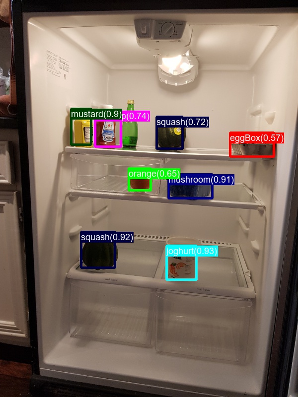
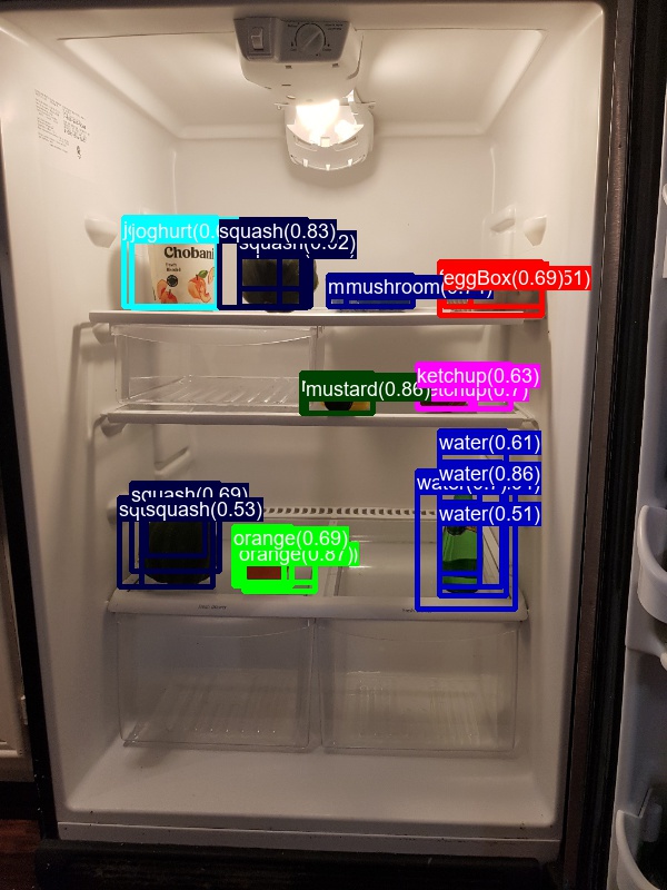
The output of the classifier using 2000 ROIs can be visualized using the script 5_visualizeResults.py. Only ROIs classified as grocery item are shown (not background), and only if the confidence in the detection is greater or above 0.5. Multiple ROIs are combined into single detections using Non-Maxima Suppression, the output of which is visualized below for the test images.
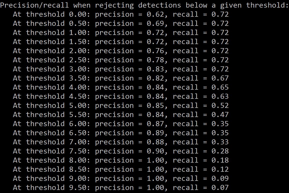
In addition to visualizing the detected objects, script 5_visualizeResults.py also computes precision and recall after rejecting detections with confidence scores less than a given threshold. This information can be used to set an operating point of the final classifier: for example, given the table below, to reach 85% precision all detections with score less than 5.0 would have to be rejected.
Script: 6_scoreImage
Up to now our focus was on training a model and evaluating its performance. Hence all steps were performed one-by-one, and intermediate results were written to and loaded from disk. During scoring, given one or more images, it would be preferable to perform all steps in-memory. Exactly this is done in script 6_scoreImage: it loads a given image, computes the ROIs, runs each ROI through the DNN, evaluates the trained SVM if needed, and finally outputs a list of the detected objects.
Note that the script makes call to functions in cntk_helpers.py which were originally written for steps 1-5. Loading the model takes a few seconds, but this only has to be done once and can then be kept in-memory (e.g. in a web-service which waits for images to be uploaded).
In part 1 we learned how to classify ROIs by training a linear Support Vector Machine on the output of a given Neural Network. We will now show how to instead perform this classification directly in the Deep Neural Network. This can be achieved by adding a new last layer which, given the input from the last fully connected layer, outputs the probabilities for each ROI to be of a certain class. See section SVM vs NN training for pros/cons of the two different approaches.
Training the Neural Network instead of an SVM is done by simply changing the variable classifier in PARAMETERS.py from "svm" to "nn". Then, as described in part 1, all the scripts need to be executed in order, except for the SVM training in step 4. This will add a classification layer to the network and train the last layer(s) of the network, and for each ROI write its classification label and confidence to disk (rather than the 4096 floats representation which was required to train the SVM). Note that NN training can cause an out-of-memory error on less powerful machines which can possibly be avoided by reducing the minibatch size and if needed also the number of ROIs per image (see variables cntk_mb_size and cntk_nrRois in PARAMETERS.py).
The mean Average Precision measure after running all steps should roughly look like the results below.
Using 200 ROIs:
| Dataset | AP(orange) | AP(eggBox) | AP(joghurt) | AP(ketchup) | mAP | |
|---|---|---|---|---|---|---|
| Test Set | 0.45 | 0.97 | 0.82 | 1.00 | 0.70 |
Using 2000 ROIs:
| Dataset | AP(orange) | AP(eggBox) | AP(joghurt) | AP(ketchup) | mAP | |
|---|---|---|---|---|---|---|
| Test Set | 1.00 | 0.92 | 1.00 | 0.07 | 0.87 |
The output of the Neural Network with 2000 ROIs on the five test images after Non-Maxima Suppression to combine multiple detections should look like this:
So far we trained and evaluated object detectors using the provided grocery dataset. It is very straight forward to use a custom dataset instead: the necessary scripts for image annotation are included in the repository, and only minor code changes are required to point to a new dataset.
First, lets have a look at the folder structure and the provided annotation files for the grocery data:
Note how all positive, negative and test images and their annotations are in the subfolders positive, negative and testImages of data/grocery/. Each image (with the exception of the negative images) has (i) a similarly named [imageName].bboxes.txt file where each row corresponds to the co-ordinates of a manually labeled object (aka. bounding box); and (ii) a [imageName].bboxes.labels.txt file where each row corresponds to the class of the object (e.g. avocado or orange).
Option #1: Visual Object Tagging Tool (Recommended)
The Visual Object Tagging Tool (VOTT) is a cross platform annotation tool for tagging video and image assets.
VOTT provides the following features:
- Computer-assisted tagging and tracking of objects in videos using the Camshift tracking algorithm.
- Exporting tags and assets to CNTK Fast-RCNN format for training an object detection model.
- Running and validating a trained CNTK object detection model on new videos to generate stronger models.
How to annotate with VOTT:
- Download the latest Release
- Follow the Readme to run a tagging job
- After tagging Export to the dataset directory
Option #2: Using Annotation Scripts
These two .txt files per image can be generated using the scripts A1_annotateImages.py and A2_annotateBboxLabels.py.
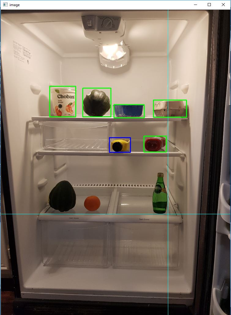
The first script lets the user draw rectangles around each object (see left image below). Once all objects in an image are annotated, pressing key 'n' writes the .bboxes.txt file and then proceeds to the next image, 'u' undoes (i.e. removes) the last rectangle, and 'q' quits the annotation tool.
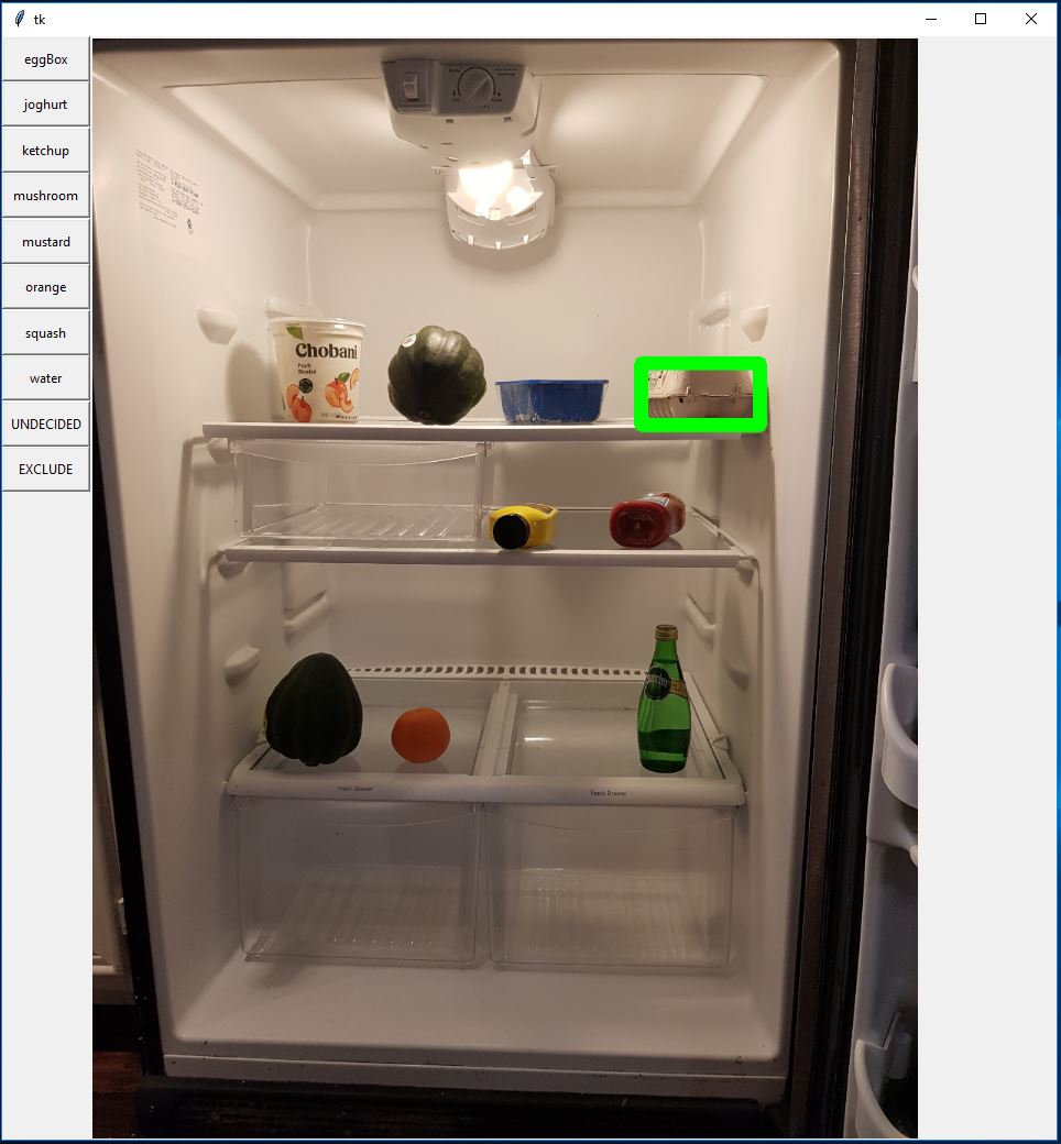
The second script loads these manually annotated rectangles for each image, displays them one-by-one, and asks the user to provide the object class by clicking on the respective button to the left of the window (see right image below). Ground truth annotations marked as either "undecided" or "exclude" are fully excluded from further processing.
If you used VOTT to generate and export your datatset, it will all ready be in sorted in to positive*, negative and testImages subfolders.
Otherwise, once all (non-negative) images are annotated using the annotation scripts, the images and .txt annotation files should be copied to the positive, negative and testImages subfolders of a new directory called data/myOwnImages/, where the string "myOwnImages" can be replaced at will.
The only required code change is to update the datasetName variable in PARAMETERS.py to the newly created folder:
datasetName = "myOwnImages"All steps in part 1 can then be executed in order and will use the new dataset.
As is true for most Machine Learning project, getting good results requires careful parameter tuning. To help with this, all important parameters are specified, and a short explanation provided, in a single place: the PARAMETERS.py file.
Here now a few tips on how to find good parameters / design a good training set:
- Select images carefully and perform annotations identically across all images. Typically, all objects in the image need to be annotated, even if the image contains many of them. It is common practice to remove such cluttered images. This is similarly true also for images where one is uncertain about the label of an object or where it is unclear whether the object should even be annotated (e.g. due to truncation, occlusion, motion blur, etc.).
- During Region-of-Interest generation in step 1, all ROIs which are deemed too small, too big, etc. are discarded. This filtering step relies on thresholds on the respective properties and are defined in
PARAMETERS.py(paragraph "ROI generation").
Visualizing the generated ROIs helps tremendously for debugging and can be done either while computing the ROIs in the script1_computeRois.pyitself, or by visualizing the CNTK training files using the scriptB2_cntkVisualizeInputs.py. In addition, scriptB1_evaluateRois.pycomputes the percentage of annotated ground truth objects that are covered by one or more ROI (i.e. recall). Generally the more ROIs (variablecntk_nrRois) the better the accuracy, but at slower training and scoring speeds. - Training a linear SVM (step 4) is relatively robust and hence for most problems the corresponding parameters in
PARAMETERS.py(paragraph "svm training") do not need to be modified. The evaluation script5_evaluateResults.pycan be used to verify that the SVM successfully learned to capture the training data (typically the APs are above 0.5). - Training a Neural Network (part 2) is significantly more difficult, and often requires expert knowledge to make the network converge to a good solution (see Michael Nielsen's great introduction to Deep Neural Networks). The arguably most important parameter here is the learning rate (parameter
cntk_lr_per_image). - In addition to computing mAP, always also visualize the results on the test and on the training set. This is done with script
5_visualizeResults.pyand helps getting an understanding of the error modes, and to verify the model is behaving as expected.
Finally, the trained model can be used to create a web service or Rest API on Azure. For this, we recommend using a technology called Flask, which makes it easy to run Python code in the cloud. See the tutorial Creating web apps with Flask in Azure for an introduction to Flask, and the GitHub repo Azure-WebApp-w-CNTK for an example how to deploy and run CNTK inside a web-service on Azure.
The last part of this tutorial shows how to reproduce published results on the Pascal VOC dataset.
First, the Pascal VOC data as well as the pre-computed Selective Search boxes need to be downloaded from these links: VOCtest_06-Nov-2007.tar, VOCtrainval_06-Nov-2007.tar, selective_search_data.tgz.
<VOC 2012 trainval http://host.robots.ox.ac.uk/pascal/VOC/voc2012/VOCtrainval_11-May-2012.tar>
<DELETE How to download the Pascal VOC 2007 and 2012 datasets is described on the Fast R-CNN page, section "Beyond the demo: installation for training and testing models". The page also describes how to download the pre-computed Selective Search boxes (using script fetch_selective_search_data.sh).>
These three tar-compressed files should to be extracted and copied into the resources/pascalVocData/ directory. Your resources folder should look like this:
resources/pascalVocData/selective_search_data
resources/pascalVocData/VOCdevkit2007/VOC2007
resources/pascalVocData/VOCdevkit2007/VOC2007/Annotations
resources/pascalVocData/VOCdevkit2007/VOC2007/ImageSets
resources/pascalVocData/VOCdevkit2007/VOC2007/JPEGImages
Second, the datasetName variable in PARAMETERS.py needs to point to the Pascal VOC dataset instead of our grocery dataset:
datasetName = "pascalVoc"Now the steps from part 1 can be executed in order with the exception of:
- Step 1: ROI generation is not necessary since we use the downloaded Selective Search boxes instead.
- Step 4: SVM training is not necessary since the classification is done by adding a new softmax layer to the network (similar to part 2).
Note that Pascal VOC is a very big dataset and hence some of the steps (especially the CNTK training in step 3) will take hours to complete.
The table below shows the mean Average Precision (mAP) of our final model, and compares this figure to the corresponding experiment in the Fast R-CNN paper (Table 6, group "S"). Note that this tutorial uses an AlexNet architecture, and we do not perform bounding box regression. To be consistent with the paper, our model is trained using the VOC 2007 "trainval" set, and the mean Average Precision is computed on the VOC 2007 "test" set.
| Dataset | mAP |
|---|---|
| Published results | 0.52 |
| Our results | 0.48 |
More information on training a PascalVOC classifier (including a download link to a trained model) can be found at CNTK's Fast-RCNN page.
R-CNNs for Object Detection were first presented in 2014 by Ross Girshick et al., and shown to outperform previous state-of-the-art approaches on one of the major object recognition challenges in the field: Pascal VOC. Since then, two follow-up papers were published which contain significant speed improvements: Fast R-CNN and Faster R-CNN.
The basic idea of R-CNN is to take a deep Neural Network which was originally trained for image classification using millions of annotated images and modify it for the purpose of object detection. The basic idea from the first R-CNN paper is illustrated in the Figure below (taken from the paper): (1) Given an input image, (2) in a first step, a large number region proposals are generated. (3) These region proposals, or Regions-of-Interests (ROIs), are then each independently sent through the network which outputs a vector of e.g. 4096 floating point values for each ROI. Finally, (4) a classifier is learned which takes the 4096 float ROI representation as input and outputs a label and confidence to each ROI.
While this approach works well in terms of accuracy, it is very costly to compute since the Neural Network has to be evaluated for each ROI. Fast R-CNN addresses this drawback by only evaluating most of the network (to be specific: the convolution layers) a single time per image. According to the authors, this leads to a 213 times speed-up during testing and a 9x speed-up during training without loss of accuracy.
The original Caffe implementation used in the R-CNN papers can be found at github: RCNN, Fast R-CNN, and Faster R-CNN. This tutorial uses some of the code from these repositories, notably (but not exclusively) for svm training and model evaluation.
In the last section, we describe how a linear SVM model is trained on the ROI 4096 float embedding. Alternatively, and this has pros/cons which are outlined below, one can do this classification directly in the neural network in a soft-max layer that takes the 4096 floats of the 2nd-to-last fully-connected layer as input.
The advantage of adding a new soft-max layer is that the full network can be retrained using backpropagation, including all convolution layers, which can lead to (slightly to moderately) better prediction accuracies. Another (implementation-dependent) advantage is that only (number of classes +1) floats per ROI need to be written to disk compared to the 4096 floats ROI embedding used to train a SVM.
On the other hand, training a Neural Network requires a good GPU, is even then 1-2 magnitudes slower than training a SVM, and requires extensive parameter tweaking and expert knowledge.
Selective Search is a method for finding a large set of possible object locations in an image, independent of the class of the actual object. It works by clustering image pixels into segments, and then performing hierarchical clustering to combine segments from the same object into object proposals. The first image in part 1 shows an example output of Selective Search, where each possible object location is visualized by a green rectangle. These rectangles are then used as Regions-of-Interests (ROIs) in the R-CNN pipeline.
The goal of ROI generation is to find a small set of ROIs which however tightly cover as many objects in the image as possible. This computation has to be sufficiently quick, while at the same time finding object locations at different scales and aspect ratios. Selective Search was shown to perform well for this task, with good accuracy to speed trade-offs.
Object detection methods often output multiple detections which fully or partly cover the same object in an image. These ROIs need to be merged to be able to count objects and obtain their exact locations in the image. This is traditionally done using a technique called Non-Maxima Suppression (NMS). The version of NMS we use (and which was also used in the R-CNN publications) does not merge ROIs but instead tries to identify which ROIs best cover the real locations of an object and discards all other ROIs. This is implemented by iteratively selecting the ROI with highest confidence and removing all other ROIs which significantly overlap this ROI and are classified to be of the same class.
Detection results before (left) and after (right) Non-maxima Suppression:
Once trained, the quality of the model can be measured using different criteria, such as precision, recall, accuracy, area-under-curve, etc. A common metric which is used for the Pascal VOC object recognition challenge is to measure the Average Precision (AP) for each class. Average Precision takes confidence in the detections into account and hence assigns a smaller penalty to false detections with low confidence. For a description of Average Precision see Everingham et. al. The mean Average Precision (mAP) is computed by taking the average over all APs.
One big item for future work is to use CNTK's Python APIs. Once these are fully available, the following changes can be made which should significantly improve run-time performance and simplify the code:
- Reduce start-up time by loading the model only once and then keeping it persistent in memory. <-- Done in v1.
- Reduce processing time using in-memory calls of the python wrappers, rather than writing all inputs and outputs to file first and subsequently parsing the CNTK output back into memory (e.g. this is especially expensive for the temporary file train.z in step 3 which can be many Gigabytes in size). <-- Done in v1.
- Reduce code complexity by evaluating the network for each ROI on-the-fly in the
im_detect()function rather than pre-computing all outputs in steps 4 and 5.
Other items for future work include:
- Replace Selective Search with a faster and more accurate implementation. <-- Done in v1.
- Adding bounding box regression.
- Implementation of faster R-CNN, i.e. performing ROI generation inside the DNN.
- Using a more recent DNN topology such as ResNet instead of AlexNet.
Patrick Buehler, Senior Data Scientist
