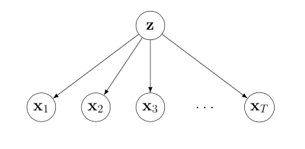
Sequential Adaptive Mixture Importance Sampling (Sequential AMIS)

This inference routine is designed to be used on static sequential models, that is, where one has a sequence of target distributions. As a point of history, it was developed for the context of a hierarchical model, where one is interested in the sequence of posterior distributions:

My personal motivation was the multi-task dynamical system, where performing efficient inference over $z$ turned out to be more challenging than expected. The graphical model takes the following form:

and particle filtering is effectively not possible, and assumed density filtering too expensive. Nevertheless, sequential AMIS may be used for any sequence of target, such as annealing between a source and target distribution.

AMIS

Calculating each posterior in the above problem uses an implementation of AMIS (Cappé et al. 2008). This procedure iteratively improves a proposal distribution via a sampling-reweighting-refitting loop. This channels the previous computation through the bottleneck of a parametric form, which avoids the re-weighting problem of using particle filtering. We use a Gaussian mixture model (GMM, similarly to Cappé et al.) with $k$ components, where the complexity can be easily tuned via choice of $k$.

There's not so many implementations of AMIS kicking around, and it appears to be an effective algorithm for many problems I've tried it on; it might therefore be of interest in its own right. For complex or high dimensional target distributions, one may wish to consider annealing from the prior. This may be easily accomplished using the sequential AMIS function below.

Implementation notes: I wrote the source for this a couple of years before this refactoring, and therefore I cannot vouch for the correctness of the code wrt the original paper. FWIW it's unlikely that there is anything major different, but it may differ in some small details.

One detail that is different is that the GMM fit at each iteration uses the previous proposal as a (weak) prior for the refined GMM. This helps avoid the usual component degeneracy issue which causes unbounded likelihoods. But it further helps in the (common) case where importance sampling results in a very low effective sample size after re-weighting (if KL(target || proposal) is large). Fitting a distribution to the resulting sample can result in a complete collapse of the proposal distribution, and the algorithm effectively gets 'stuck'. This is avoided by use of conjugate priors (Dirichlet, NormalInverseWishart) which provide additional 'pseudo-observations'.

Syntax (dumped from the docstring):

    amis(log_f, pis, mus, covs; nepochs=5, gmm_smps=1000, IS_tilt=1., terminate=0.75, debug=false)

    amis(log_f, S, k::Int; nepochs=5, gmm_smps=1000, IS_tilt=1., terminate=0.75, debug=false)

    amis(log_f, S, W, k::Int; nepochs=5, gmm_smps=1000, IS_tilt=1., terminate=0.75, debug=false)

(1) log_f: the target function (distribution). This should take a single argument: a set of $n \times d$ samples, and return a vector of length $n$ of the log of the unnormalized target function (distribution) for each sample.

(2) pis: $k$-length probability vector of probabilities of each cluster.

(3) mus: matrix of cluster means: each row is a mean vector.

(4) covs: batched covariance matrices stacked in Tensor d×d×k for $k$ clusters.

Instead of args (2-4), i.e. the parameters of the GMM, one can instead supply a matrix S of $n$ initial samples ($n \times d$ matrix), and optionally a $n$-length vector W of log weights corresponding to each sample. In this case, one must supply an integer $k$ (for the GMM components) as a final positional argument.

Return value This function returns a MCPosterior struct which contains a matrix of samples (.samples) and a vector of log weights (.logW). We provide a few helper methods such as weights(.) for (normalized) per-sample weights, ess(.) to calculate the Effective Sample Size and resample(., N) to resample N samples from the discrete posterior.

Sequential AMIS

The sequential AMIS routine exploits the proposal distribution learned at time $t-1$ as the initial proposal at time $t$. This can have a useful annealing effect. It is not difficult to code up this sequential procedure using the AMIS routine above, but there are a couple of useful additions implemented here, not least retrying AMIS with different parameters when the effective sample size becomes too low.

The function seq_amis:

seq_amis(target_logfs, init_dist::Union{Distribution, Int}, k::Int; nepochs=4, IS_tilt=1.3f0,
                  gmm_smps=2000, terminate=0.6, max_retry=3, verbose=true, min_ess=min(100, gmm_smps/2))

takes a vector (or other iterable) of target log densities (these may be unnormalized, as above), an initial distribution (one can supply simply the dimension of the problem to use the default of a standard multivariate Gaussian), and the number of GMM components, $k$.

Example Usage

A simple example, using Gaussian targets is shown below. If you haven't, instantiate the environment, e.g. via

activate .
instantiate

Then run the test script (include("test/runtests.jl")) or if you'd prefer an interactive session, run the following commands:

using Distributions: MvNormal, logpdf
using SeqAdaptiveIS

n_targets = 8
true_pars = [(zeros(2) .+ i, Float64[1 0; 0 1] ./ i) for i in 1:n_targets];
seq_targets = [x->logpdf(MvNormal(μ, Σ), x') for (μ, Σ) in true_pars]
prior = MvNormal(zeros(2), Float64[1 0; 0 1])

seq_smps, seq_gmms = seq_amis(seq_targets, prior, 3)
# which is equivalent to seq_amis(seq_targets, 2, 3)

# test e.g.
mean(seq_samps[8].samples, dims=1) # ~= [8,8]

For those unfamiliar with Julia, note that the first function call will hit the Just-Ahead-of-Time compiler, and incur a substantial delay before running.

ornithos/SeqAdaptiveIS

Sequential Adaptive Mixture Importance Sampling (Sequential AMIS)

AMIS

Sequential AMIS

Example Usage