MTDS for Double Pendulum

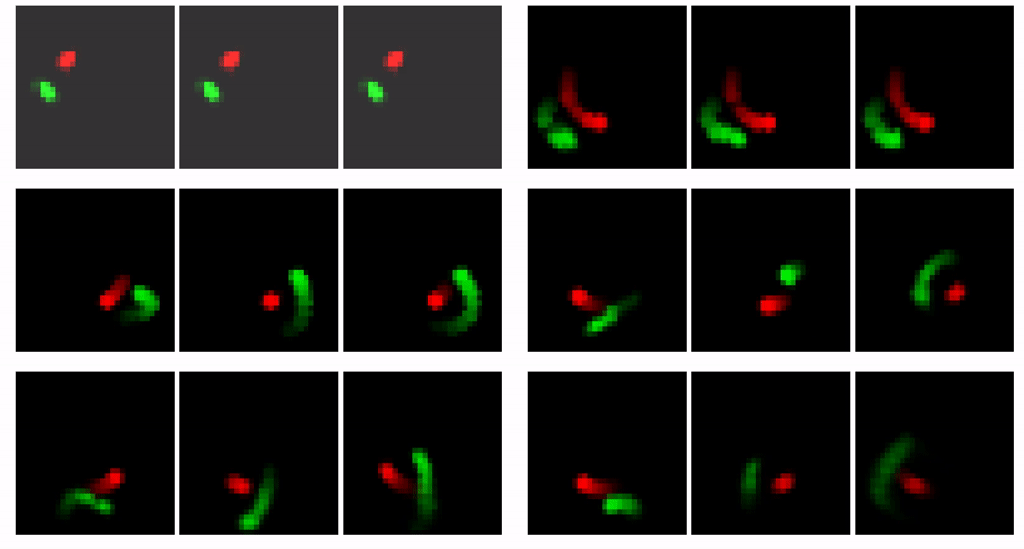
MTDS applied to video data of a double pendulum. This is code for the updated MTDS project -- for the previous version of the paper see https://arxiv.org/abs/1910.05026. The details for the double pendulum work are only available in the updated paper which is currently under review. This repo is therefore not yet properly packaged up for an end user, although it will not take much extra work. For those who are interested, the code is fairly well annotated, and there's some commands to get you started below.

Our goal here is to show that by changing the architecture to an MTDS construct, we can permit customizable predictions from a seq2seq RNN (with convolutional encoder/decoder). An example is shown below. Here, the prediction for the first 10 frames is identical (shown with the lighter grey), after which we adjust the latent variable to yield three possible predictions.

For more examples, with some commentary, see https://sites.google.com/view/mtds-customized-predictions/home.

Example code usage

In this example, we load a pre-trained model (please download the data repository from https://gin.g-node.org/alxbird/dblpendulum -- note that the CLI appears not to work for downloading this file, at least if you're not logged into gin, so just download it directly from the webpage. Unpack the data into a folder called data within the structure of this repo. (YAML files in saved_models will point here.)

Imports / compile code

using Flux

# Load MTDS libraries
include("src/modelutils.jl")
include("src/datagen.jl")
include("src/seq2seq.jl")
include("src/multitask.jl")

const unsqueeze = modelutils.unsqueeze;  # trivial but useful function
const chan3cat = modelutils.chan3cat     # concatenate with (zero) 3rd colour channel
standardize(x; dims=1) = (x .- mean(x; dims=dims)) ./ std(x; dims=dims);
make_untracked(x) = mapleaves(Tracker.data, x)   # remove AD

Generate data

data_xy, data_θ, data_meta = datagen.generate_data();   # _seed argument is fixed, but can be changed

# data_xy   - (x,y) co-ordinates of bob1 and bob2.
# data_θ    - (θ, θdot) state of bob1 and bob2 (for reference, but unused in model).
# data_meta - metadata about each sequence incl. ODE parameters and initial conditions.

# To reduce memory usage, we won't "image" all of these co-ordinates for the videos
# but instead construct these "on-demand". Julia can do this in microseconds.
constr_image(x) = (@assert length(x) == 4; datagen.gen_pic_circ2_2chan_cood_tf(x[1:2], x[3:4]))

tT = 80
cseq = [unsqueeze(constr_image(data_xy[:test][10][tt, :]), 4) for tt in 1:tT] # |> gpu # for loading to GPU.

Load previously trained model

video_mtgru_pred_fixb_u = mtmodel.load_model_from_def("saved_models/mtgru_video_fixb_pred_300.yml")
video_mtgru_pred_fixb_u = make_untracked(video_mtgru_pred_fixb_u)  # |> gpu # for loading to GPU.

Predict example test sequence

# Predict forward `T_steps` from the first `T_enc` values of the current sequence (`cseq`).
# Note that the prediction is in logits, and we must transform to [0,1] via sigmoid.
logit_yhat = video_mtgru_pred_fixb_u(cseq; T_enc=20, T_steps=80)
yhat = map(x->σ.(x), logit_yhat);    # perform (elementwise) sigmoid transform to list

Performing inference of latent z

Extract the mean embedding of x0 for the relevant sequences

We extract all of the initial x0 variables for each sequence in the test set. (This is quick, and amortizes the cost incurred otherwise from each sample of z. The code is similar to above, but see ?mtmodel.posterior_samples for more details.

# initial x0 of test set
m = video_mtgru_pred_fixb_u
testx0 = []
for i = 1:10
    cbatch = (10*(i-1)+1):10*i
    cseqs = Flux.batch([data_xy[:test][s][1:10,:] for s in cbatch])
    cseqs = [cat([datagen.gen_pic_circ2_2chan_cood_tf(cseqs[tt, 1:2, s], cseqs[tt, 3:4, s])
                for s in 1:10]..., dims=4) for tt in 1:10]; # [32×32×2×nbatch for t in 1:70].
    post = mtmodel.posterior_samples(m, cseqs, []; z=0, c=0, T_enc=20)
    push!(testx0, (post[2][1], post[3][1]))
end

testx0 = (reduce(hcat, [x[1] for x in testx0]), reduce(hcat, [x[2] for x in testx0]))
testx0post = [MvNormal(testx0[1][:,i], Diagonal(testx0[2][:,i].^2)) for i in 1:100];

Create some useful structs to retain the samples

This is not essential, but tidies up the results later.

using NNlib

struct MCPosterior
    samples::AbstractMatrix
    logW::Vector
    ess::AbstractFloat
end

weights(P::MCPosterior) = NNlib.softmax(P.logW)
resample(P::MCPosterior, N::Int) = P.samples[rand(Categorical(weights(P)), N),:]
Base.length(P::MCPosterior) = length(P.logW)
ess(P::MCPosterior) = P.ess

struct GMM{T <: Real}
    pis::Vector{T}
    mus::AbstractMatrix{T}
    covs::AbstractArray{T}
end

Specify prior distributions for z

These are calculated based on the aggregate posterior of the training set, but we take a shortcut here:

pzmean, pzcov = Float32[-0.012118647, 0.18318911], Float32[0.187806 0.0241003; 0.0241003 0.230048];
p_z = MvNormal(pzmean, pzcov)

Generator function: creates log joint function for a given test_ix and time.

function generate_logjoint(m, test_ix, to_time, data_xy, p_z; batch_size=15, β_def=1f0)
    x0 = trainx0post[test_ix].μ
    function logjoint(S, β=β_def)
        # β for annealing
        bsz = batch_size
        n, d = size(S)
        @argcheck d == 2

        y = data_xy[tvt][test_ix][1:to_time,:]
        y = [datagen.gen_pic_circ2_2chan_cood_tf(y[tt, 1:2], y[tt, 3:4])
                for tt in 1:to_time]; # [32×32×2 for t in 1:to_time].
        Z = gpu(S[:, 1:2]')
        nllh = map(Iterators.partition(1:n, bsz)) do cbatch
            x0_init = gpu(repeat(x0, 1, length(cbatch)))  # using mean posterior x0
            txb = mtmodel.online_inference_BCE(m, x0_init, Z[:, cbatch], y)
            cpu(dropdims(sum(txb, dims=1), dims=1))   # online BCE result is T × batchsize; sum over time
        end
        llh = - reduce(vcat, nllh)
        # prior
        lp_z = logpdf(p_z, cpu(Z))
        return  lp_z + β*llh
    end
end

Run inference for t = 5,10,15,20

test_ix = 5

smp_out = []
dist_out = []

k = 3
nepochs = 3
gmm_smps = 2000
t0 = time()
t_begin = copy(t0)
printfmtln("========= TEST INDEX {:d} ========", test_ix)
S, logW, pis, mus, covs = nothing, nothing, nothing, nothing, nothing  # local scope
for t in 5:5:20
    IS_tilt, nepochs, c_ess = 1.3f0, 3, 0
    if t==5
        for j = 1:3
            lj = generate_logjoint(video_mtgru_u, test_ix, t, data_xy, p_z, p_c_0; batch_size=10, β_def=1f0)
            S, logW, pis, mus, covs = infer.amis(lj, MvNormal(vcat(p_z.μ, p_c_0.μ),
                    Diagonal(vcat(diag(p_z.Σ), diag(p_c_0.Σ)))), k; nepochs=nepochs, gmm_smps=gmm_smps)
            c_ess = infer.eff_ss(softmax(logW))
            (c_ess > 100) && break
            IS_tilt, nepochs = IS_tilt*1.3, nepochs + 1
            println("Retrying...")
        end
    else
        for j in 1:3
            lj = generate_logjoint(video_mtgru_u, test_ix, t, data_xy, p_z, p_c_0; batch_size=50, β_def=1f0)
            S, logW, pis, mus, covs = infer.amis(lj, pis, mus, covs, S, logW; nepochs=nepochs,
                gmm_smps=gmm_smps, IS_tilt=1.3)
            c_ess = infer.eff_ss(softmax(logW))
            (c_ess > 100) && break
            IS_tilt, nepochs = IS_tilt*1.3, nepochs + 1
            println("Retrying...")
        end
    end
    push!(smp_out, MCPosterior(S, logW, c_ess))
    push!(dist_out, (pis, mus, covs))
    printfmtln("Posterior {:d}, ess={:.2f}, time taken = {:.2f}s ({:.2f}).", t, c_ess,
        time()-t_begin, time() - t0); flush(stdout);
    t0 = time()
end

ornithos/mtds-dblpend