Class Imbalance Problems - Lab

Introduction

Now that you've gone over some techniques for tuning classification models on imbalanced datasets, its time to practice those techniques. In this lab, you'll investigate credit card fraud and attempt to tune a model to flag suspicious activity.

Objectives

You will be able to:

Use modified sampling techniques to address class imbalance problems
Understand the complications of class imbalance problems

Predicting Credit Card Fraud

Load the creditcard.csv.gz file and preview the data. To load a compressed csv use the optional parameter compression='gzip' within pandas read_csv method as in: pd.read_csv(filename, compression='gzip').

#Your code here

Preview the class imbalance

You should see that the dataset has 31 columns. The first is a time field followed by V1-V28, created by way of manual feature engineering done on the backend that we have little information about. Finally, there's the amount of the purchase and a binary Class flag. This last column, Class, is the indication of whether or not the purchase was fraudulent, and it is the feature you should be attempting to predict.

Take a look at how imbalanced this dataset is.

#Your code here

Define the Problem

Define X and y and perform a standard train test split.

#Your code here

Create an initial model

As a baseline, fit a cookie cutter out of the box logistic regression model. Then plot the ROC curve and print out the AUC. We'll use this as a comparison for how our future models perform.

#Your code here

Tuning

Try some of the various techniques proposed to tune your model. Compare your models using AUC, ROC or another metric.

#Your code here

SMOTE

If you haven't already, try using the SMOTE class from the imblearn package in order to improve the model's performance on the minority class.

#Your code here

Analysis

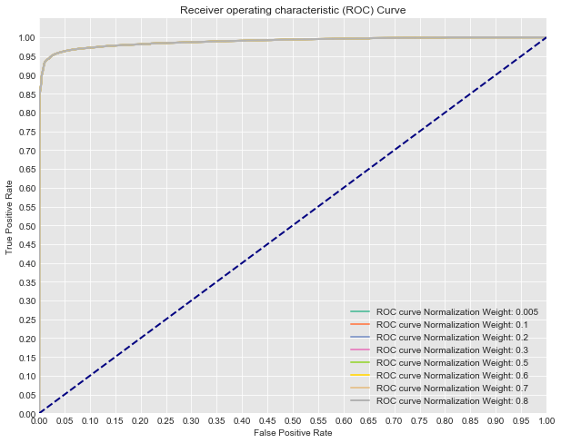
Describe what is misleading about the AUC score and ROC curves produced by this code:

print(y.value_counts()) #Previous original class distribution
X_resampled, y_resampled = SMOTE().fit_sample(X, y) 
print(pd.Series(y_resampled).value_counts()) #Preview synthetic sample class distribution

X_train, X_test, y_train, y_test = train_test_split(X_resampled, y_resampled, random_state=0)

# Now let's compare a few different regularization performances on the dataset:
C_param_range = [0.005, 0.1, 0.2, 0.3, 0.5, 0.6, 0.7, 0.8]
names = [0.005, 0.1, 0.2, 0.3, 0.5, 0.6, 0.7, 0.8, 0.9]
colors = sns.color_palette("Set2", n_colors=len(names))

plt.figure(figsize=(10,8))

for n, c in enumerate(C_param_range):
    #Fit a model
    logreg = LogisticRegression(fit_intercept = False, C = c) #Starter code
    model_log = logreg.fit(X_train, y_train)
    print(model_log) #Preview model params

    #Predict
    y_hat_test = logreg.predict(X_test)

    y_score = logreg.fit(X_train, y_train).decision_function(X_test)

    fpr, tpr, thresholds = roc_curve(y_test, y_score)
    
    print('AUC for {}: {}'.format(names[n], auc(fpr, tpr)))
    lw = 2
    plt.plot(fpr, tpr, color=colors[n],
             lw=lw, label='ROC curve Normalization Weight: {}'.format(names[n]))
plt.plot([0, 1], [0, 1], color='navy', lw=lw, linestyle='--')
plt.xlim([0.0, 1.0])
plt.ylim([0.0, 1.05])

plt.yticks([i/20.0 for i in range(21)])
plt.xticks([i/20.0 for i in range(21)])
plt.xlabel('False Positive Rate')
plt.ylabel('True Positive Rate')
plt.title('Receiver operating characteristic (ROC) Curve')
plt.legend(loc="lower right")
plt.show()

0    284315
1       492
Name: Class, dtype: int64
1    284315
0    284315
dtype: int64
LogisticRegression(C=0.005, class_weight=None, dual=False,
          fit_intercept=False, intercept_scaling=1, max_iter=100,
          multi_class='ovr', n_jobs=1, penalty='l2', random_state=None,
          solver='liblinear', tol=0.0001, verbose=0, warm_start=False)
AUC for 0.005: 0.9889222836885252
LogisticRegression(C=0.1, class_weight=None, dual=False, fit_intercept=False,
          intercept_scaling=1, max_iter=100, multi_class='ovr', n_jobs=1,
          penalty='l2', random_state=None, solver='liblinear', tol=0.0001,
          verbose=0, warm_start=False)
AUC for 0.1: 0.9889243265712433
LogisticRegression(C=0.2, class_weight=None, dual=False, fit_intercept=False,
          intercept_scaling=1, max_iter=100, multi_class='ovr', n_jobs=1,
          penalty='l2', random_state=None, solver='liblinear', tol=0.0001,
          verbose=0, warm_start=False)
AUC for 0.2: 0.9889243770445593
LogisticRegression(C=0.3, class_weight=None, dual=False, fit_intercept=False,
          intercept_scaling=1, max_iter=100, multi_class='ovr', n_jobs=1,
          penalty='l2', random_state=None, solver='liblinear', tol=0.0001,
          verbose=0, warm_start=False)
AUC for 0.3: 0.9889243972338857
LogisticRegression(C=0.5, class_weight=None, dual=False, fit_intercept=False,
          intercept_scaling=1, max_iter=100, multi_class='ovr', n_jobs=1,
          penalty='l2', random_state=None, solver='liblinear', tol=0.0001,
          verbose=0, warm_start=False)
AUC for 0.5: 0.9889244075264833
LogisticRegression(C=0.6, class_weight=None, dual=False, fit_intercept=False,
          intercept_scaling=1, max_iter=100, multi_class='ovr', n_jobs=1,
          penalty='l2', random_state=None, solver='liblinear', tol=0.0001,
          verbose=0, warm_start=False)
AUC for 0.6: 0.9889244102975672
LogisticRegression(C=0.7, class_weight=None, dual=False, fit_intercept=False,
          intercept_scaling=1, max_iter=100, multi_class='ovr', n_jobs=1,
          penalty='l2', random_state=None, solver='liblinear', tol=0.0001,
          verbose=0, warm_start=False)
AUC for 0.7: 0.9889244188087539
LogisticRegression(C=0.8, class_weight=None, dual=False, fit_intercept=False,
          intercept_scaling=1, max_iter=100, multi_class='ovr', n_jobs=1,
          penalty='l2', random_state=None, solver='liblinear', tol=0.0001,
          verbose=0, warm_start=False)
AUC for 0.8: 0.9889244061409412

Your response here

Summary

In this lab, you got some hands-on practice tuning logistic regression models using various techniques and parameters. In the upcoming labs and lessons, you will continue to dig into the underlying mathematics of logistic regression, taking on a statistical point of view and providing you with a deeper understanding of how the algorithm works. This should give you further insight as to how to tune and apply these models going forward.

ortsed/dsc-class-imbalance-problems-lab-dc-ds-career-042219