The goals / steps of this project are the following:
- Compute the camera calibration matrix and distortion coefficients given a set of chessboard images.
- Apply a distortion correction to raw images.
- Use color transforms, gradients, etc., to create a thresholded binary image.
- Apply a perspective transform to rectify binary image ("birds-eye view").
- Detect lane pixels and fit to find the lane boundary.
- Determine the curvature of the lane and vehicle position with respect to center.
- Warp the detected lane boundaries back onto the original image.
- Output visual display of the lane boundaries and numerical estimation of lane curvature and vehicle position.
1. Briefly state how you computed the camera matrix and distortion coefficients. Provide an example of a distortion corrected calibration image.
The code for this step is contained in the Camera Calibration and Distortion Correction section of the IPython notebook located in ALane.ipynb.
Using cv2.findChessboardCorners, the corners points are stored in an array imgpoints for each calibration image where the chessboard could be found. Here I am assuming the chessboard is fixed on the (x, y) plane at z=0, such that the object points are the same for each calibration image.
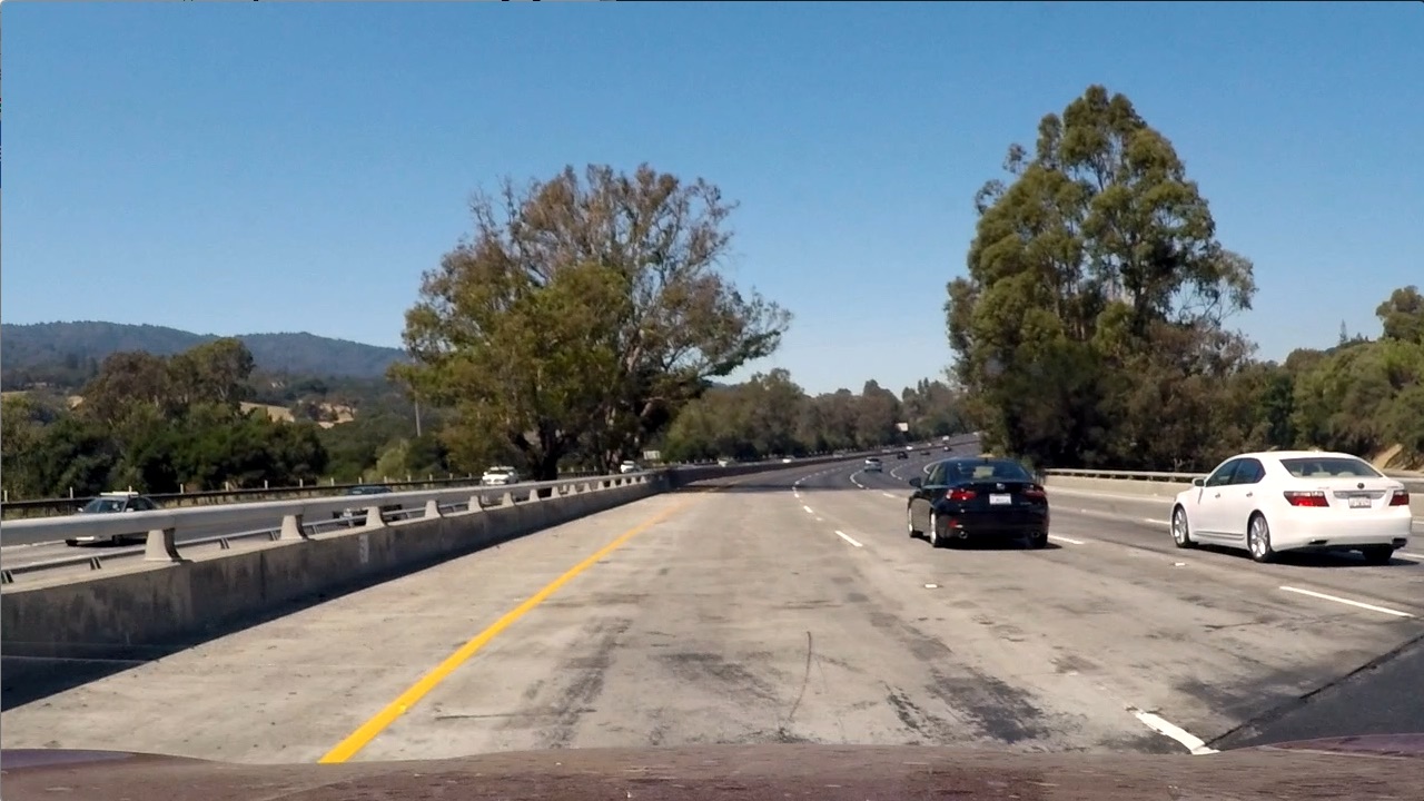
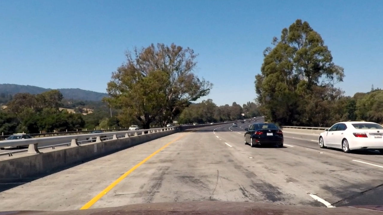
objpoints and imgpoints are used to compute the camera calibration and distortion coefficients using the cv2.calibrateCamera() function. Then cv2.undistort() function is used to obtain the following result:
Distorted image:
Distortion-corrected image:
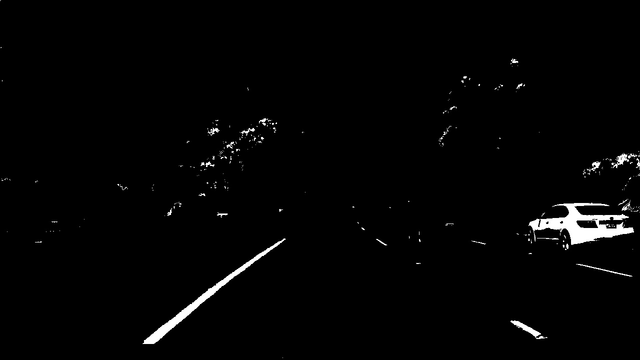
2. Describe how (and identify where in your code) you used color transforms, gradients or other methods to create a thresholded binary image. Provide an example of a binary image result.
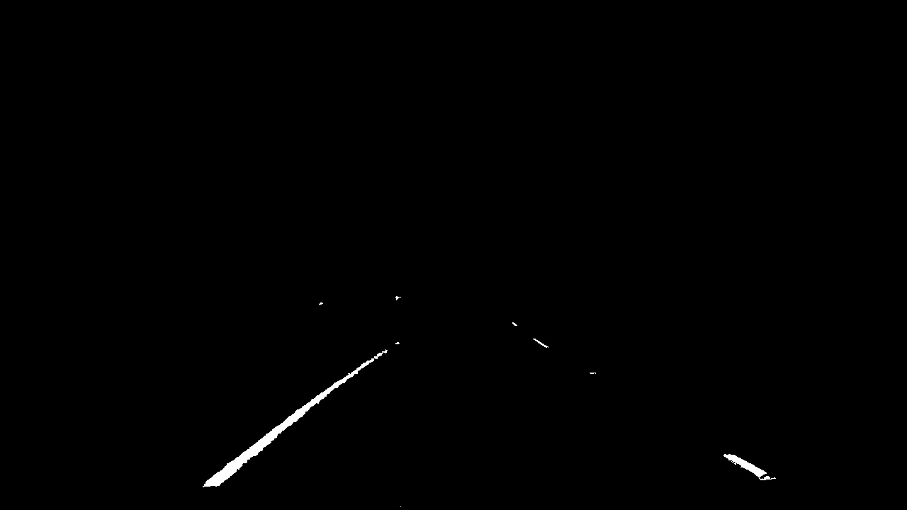
A combination of color and gradient thresholds was used to generate a binary image. Color theresholding for yellow and white lanes was done in HSV space then HLS. S and L channel was used. Gardient was computed along x direction. The code for these filters is present in the heading Binary Image. L channel in LUV with upper and lower thresholds of 255 has been added.
After Selecting Region:
3. Describe how (and identify where in your code) you performed a perspective transform and provide an example of a transformed image.
The code for perspective transform is included in a function called transformation_matrix(). The function takes as inputs an image (img). After having poor results with lane coordinates, I decided to use predefined coordinates.
src = np.float32([
    [585,460],
    [203,720],
    [1127,720],
    [695,460]])
dst = np.float32([
    [320,0],
    [320,720],
    [960,720],
    [960,0]])
This resulted in the following source and destination points:
| Source | Destination |
|---|---|
| 585, 460 | 300, 0 |
| 203, 720 | 320, 100 |
| 1127, 720 | 960, 720 |
| 695, 460 | 960, 0 |
Example:
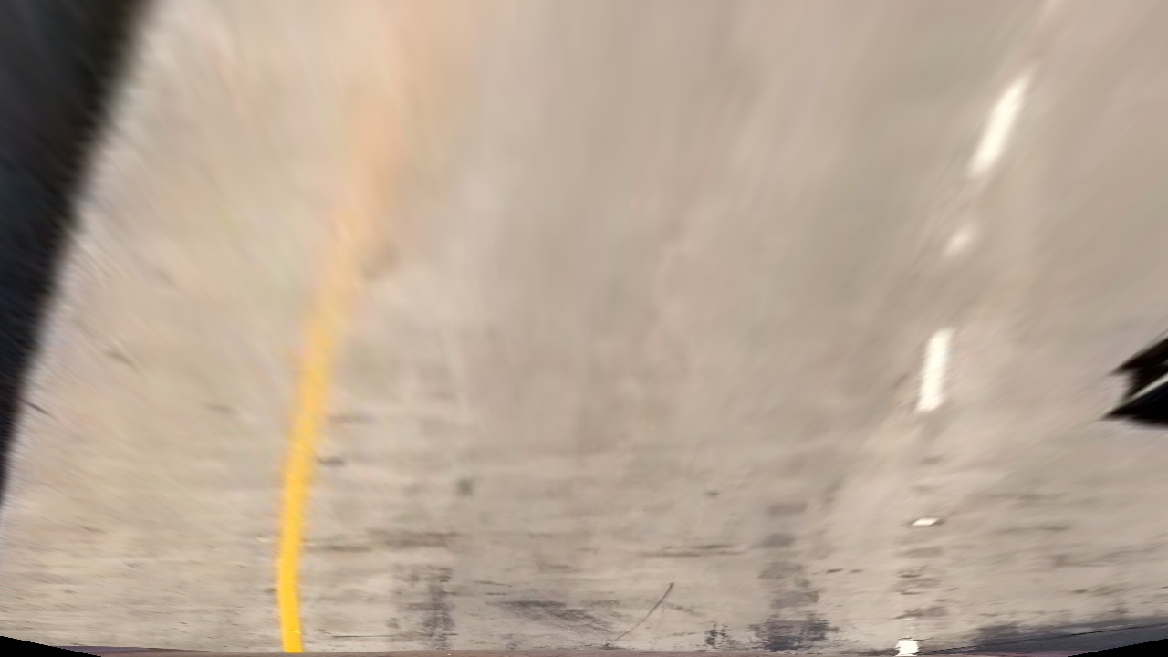
Warped image:
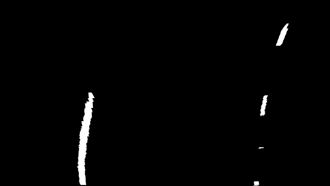
Binary warped image:
4. Describe how (and identify where in your code) you identified lane-line pixels and fit their positions with a polynomial?
In the Identifying lane-line pixels heading the get_lane_px searches for lane pixels using a sliding size of 50px and base coordinates of a lane.
    margin = 100
    nwindows = 9
    window_height = np.int(image.shape[0]/nwindows)
    leftx_current = left_base #[0]
    rightx_current = right_base#[0]
    minpix = 50 #min pixel found in each window
    left_lane_inds = []
    right_lane_inds = []

    nonzero = image.nonzero()
    nonzeroy = np.array(nonzero[0])
    nonzerox = np.array(nonzero[1])

    for window in range(nwindows):
        win_y_low = image.shape[0] - (window+1)*window_height
        win_y_high = image.shape[0] - (window*window_height)
        win_xleft_low = leftx_current - margin
        win_xleft_high = leftx_current + margin
        win_xright_low = rightx_current - margin
        win_xright_high = rightx_current + margin

        good_left_inds = ((nonzeroy >= win_y_low) & (nonzeroy < win_y_high) & (nonzerox >= win_xleft_low)\
                          & (nonzerox < win_xleft_high)).nonzero()[0]
        good_right_inds = ((nonzeroy >= win_y_low) & (nonzeroy < win_y_high) & (nonzerox >= win_xright_low)\
                          & (nonzerox < win_xright_high)).nonzero()[0]
        left_lane_inds.append(good_left_inds)
        right_lane_inds.append(good_right_inds)

        if len(good_left_inds) > minpix:
            leftx_current = np.int(np.mean(nonzerox[good_left_inds]))
        if len(good_right_inds) > minpix:
            rightx_current = np.int(np.mean(nonzerox[good_right_inds]))
    left_lane_inds = np.concatenate(left_lane_inds)
    right_lane_inds = np.concatenate(right_lane_inds)
The output looks like this:
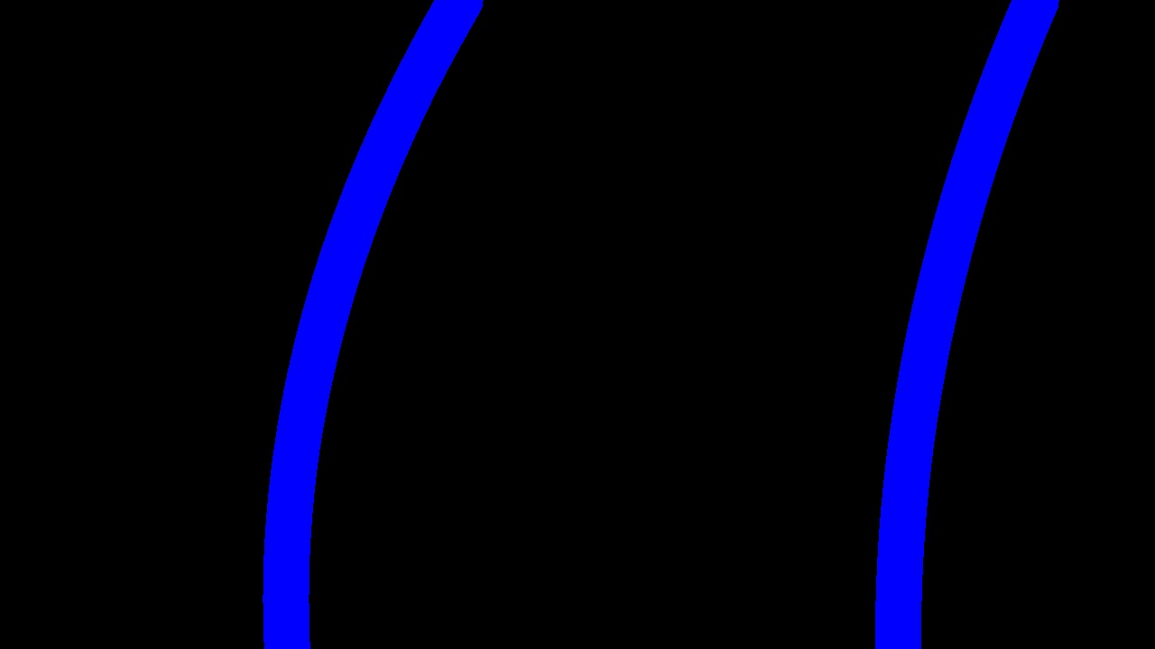
The draw_curves uses a second order polynomial to fit lane pixels.
Result:
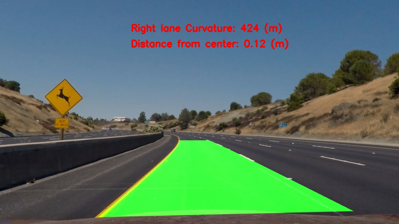
Then using the lane lines draw_lanes plots the lane.
Result:
5. Describe how (and identify where in your code) you calculated the radius of curvature of the lane and the position of the vehicle with respect to center.
The radius of curvature and the position of the vehicle with respect to center is calculated upon calling the get_curvature in sixth code cell
For a second order polynomial f(y)=A y^2 +B y + C the radius of curvature is given by R = [(1+(2 Ay +B)^2 )^3/2]/|2A|.
The distance from the center of the lane is calculated by measuring the distance to each lane and calculating the position assuming the lane has a given fixed width of 3.7m.
6. Provide an example image of your result plotted back down onto the road such that the lane area is identified clearly.
1. Provide a link to your final video output. Your pipeline should perform reasonably well on the entire project video (wobbly lines are ok but no catastrophic failures that would cause the car to drive off the road!).
Here's a link to my video result
1. Briefly discuss any problems / issues you faced in your implementation of this project. Where will your pipeline likely fail? What could you do to make it more robust?
-
The video output has the right lane boundary is skewed in some frames. This might be due to missing lane markers after prespetive transform is calculated, which offsets the polymonial fit.
-
The pipline need to be optimized as there are alot of repetitive calculations.
-
Laplacian or other gradients could be used to improve line detection.


