Teeth Recognition from image comparison

Repository to collect the code used to implement an image feature comparison.

Installation instructions

To not mess up with versioning and package installation, we strongly advice to create a virtual environment. One can follow this guide and the suitable section according to the OS.

Once the virtual environment has been set up, as usual, one has to run the following instruction from a command line

  pip install -r requirements.txt

This installs all the packages the code in this repository needs.

Introduction and motivations

The main goal is to apply such algorithm, firstly implemented to compare generic images features, to recognise teeth characteristics. This would have several important applications of high importance, e.g. the identification of people from the dental features.

The main idea is to create a library collecting methods from openCV, to make comparison between images to identify subjects up to a certain level of confidence.

Mass disaster and other applications

A motivational example might be the following: imagine the case of a mass disaster. In such an event it is crucial the precise and rapid identification of victims, a process that can be quite complicate. An image comparison system might help the forensic odontologist to compare hundreds of radiographs and find the one with highest similarity score with the given one.

An image from one of the most famous mass disasters in hystory: $11^\mathrm{th}$ September 2001.

However a model like this might be useful for many other reasons: e.g. age estimation from dental radiographs, it might help dentists to study the evolution of a disease, etc.

Shape recognition in images

Object recognition is one of the main topics in computer vision. The possibility to program or train a machine to recognise an object amongst others in an image is somehow the holy graal of this reseach area. Indeed, the literature in the field is particularly rich and abundant.

Scale-Invariant Feature Transform

The aim of this section is to answer the question

what is SIFT?

Well, SIFT -- which stands for Scale Invariant Feature Transform -- is a method for extracting feature vectors that describe local patches of an image.

These feature vectors do not only enjoy the nice property of being scale-invariant, but they are also invariant to translation, rotation, and illumination. In other words: everything a descriptor should be!

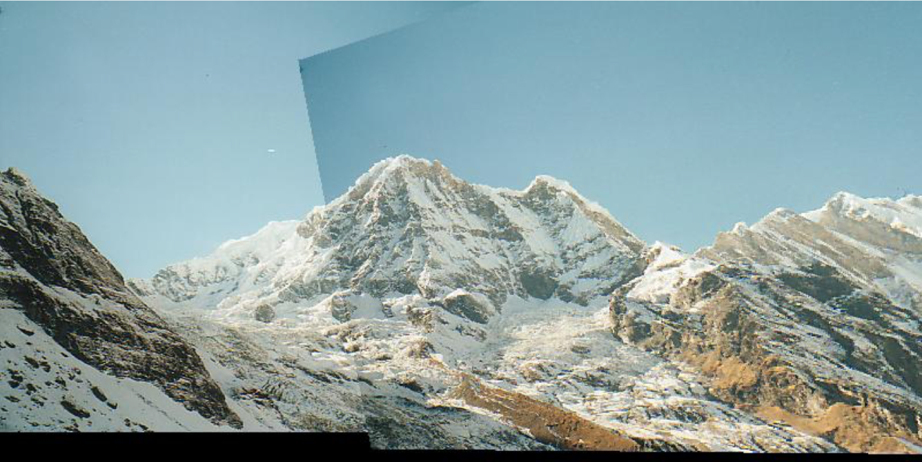
These descriptors are useful for matching objects are patches between images. For example, consider creating a panorama. Assuming each image has some overlapping parts, you need some way to align them so we can stitch them together. If we have some points in each image that we know correspond, we can warp one of the images using a homography. SIFT helps with automatically finding not only corresponding points in each image, but points that are easy to match.

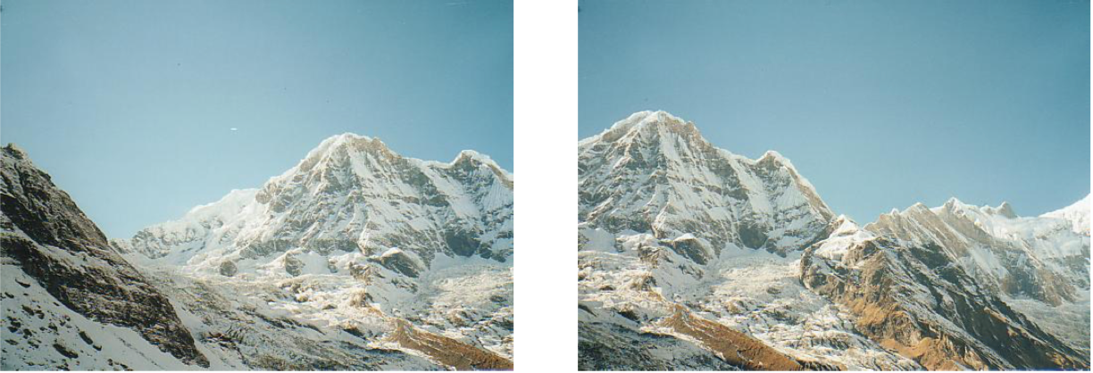
Images with overlapping regions: before and after SIFT homography.

The algorithm

One can find the many algorithm descriptions in the internet -- Wikipedia has a page dedicated to SIFT -- or reading the original Lowe's paper. Here, we give a brief description focusing on the aspects useful for our purposes. First of all, we can split the algorithm in four main steps

Scale-space building and extrema detection
Keypoint localisation
Orientation assignement
Local descriptors creation

We are going to describe each of them to just have in mind how it works. In order to implement and use the algorithm, however, we will not need all these details.

To begin, for any object in an image, interesting points on the object can be extracted to provide a "feature description" of the object. This description, extracted from a given image, can then be used to identify the object when attempting to locate the object in a second image containing possibly many other objects. As said, to perform reliable recognition, it is important that the features extracted from the training image be detectable even under changes in image scale, noise and illumination. Such points usually lie on high-contrast regions of the image, such as object edges.

The SIFT descriptor is based on image measurements in terms of receptive fields over which local scale invariant reference frames are established by local scale selection.

Constructing the scale space

Keypoints to identify are defined as extrema of a Gaussian difference in a scale space defined over a series of smoothed and resampled images.

Hence, to begin we need to define a scale space and ensure that the keypoints we are going to select will be scale-independent. In order to get rid of the noise of the image we apply a Gaussian blur, while the characteristic scale of a feature can be detected by a scale-normalised Laplacian of Gaussian (LoG) filter. In a plot, a LoG filter looks like this:

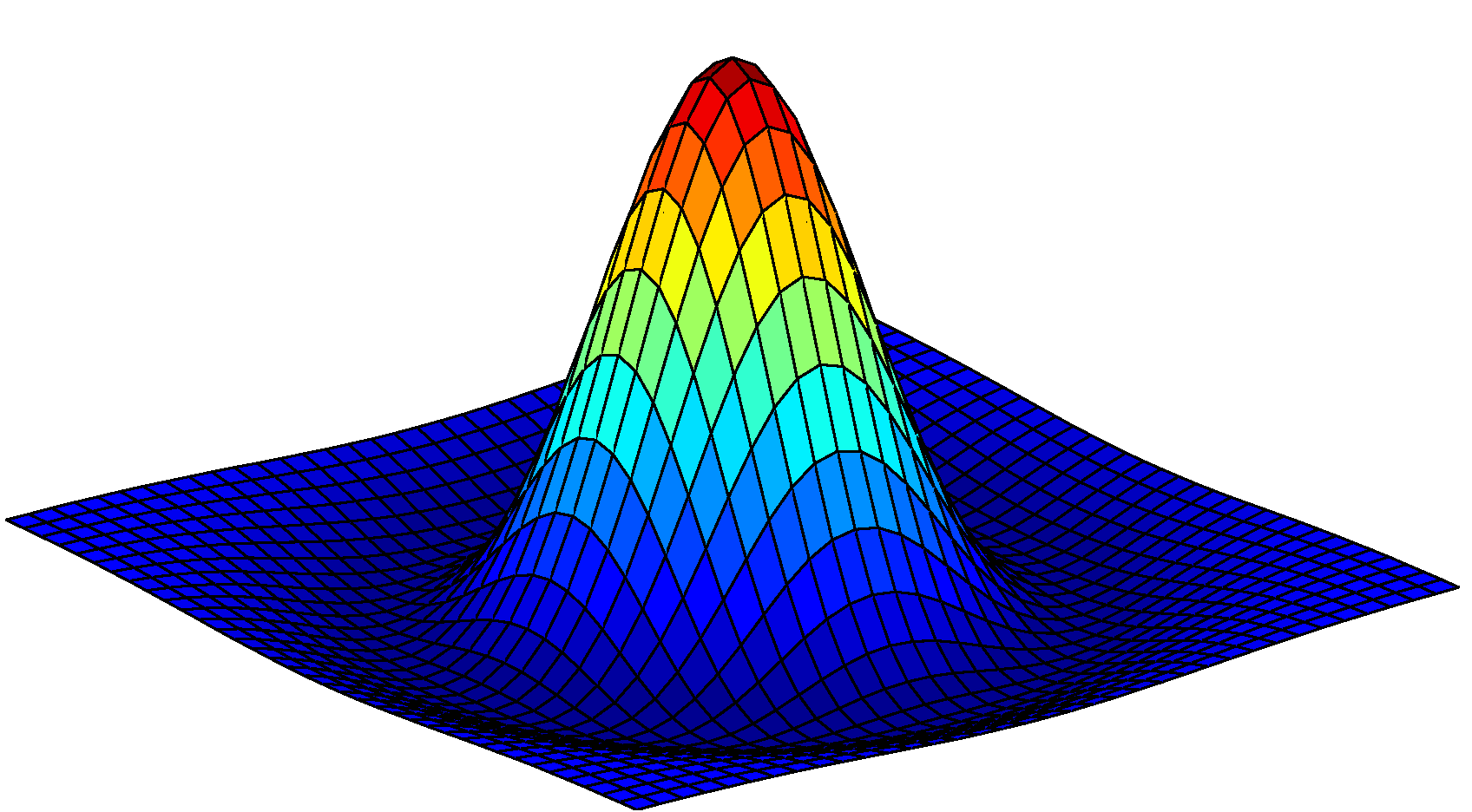
As one can observe, the LoG filter is highly peaked at the center while becoming slightly negative and then zero at a distance from the center characterized by the standard deviation $\sigma$ of the Gaussian.

The scale-normalisation for the LoG filter correspond to $\sigma^2 \textrm{LoG}$ and it is used to correct the behaviour of the response of the LoG filter for a wider Gaussian that would be lower than for a smaller $\sigma$ Gaussian.

The main issue with such a filter is that is expensive from a computationally point of view, this is due to the fact of the presence of different scales. Thankfully, even originally in the paper, the authors of SIFT came up with a clever way to efficiently calculate the LoG at many scales.

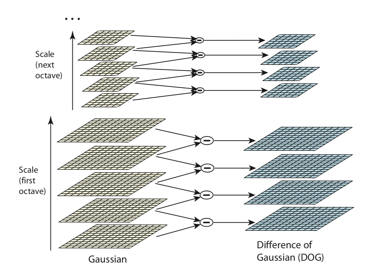
It turns out that the difference of two Gaussians (or Dog) with similar variance yields a filter that approximates the scale-normalized LoG very well:

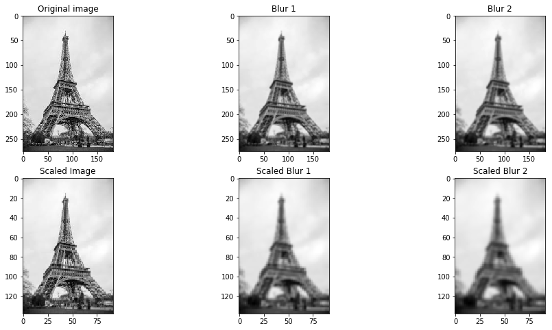
Thus, we have seen how such approximation gives us an efficient way to estimate the LoG. Now, we need to compute it at multiple scales. SIFT uses a number of octaves to calculate the DoG. Most people would think that an octave means that eight images are computed. However, an octave is actually a set of images were the blur of the last image is double the blur of the first image.

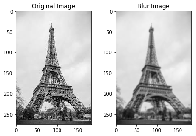
All these filters and scales will multiply the number of images to consider - or better, the number of versions of the same image. At the end of the process we will end up with blur (Gaussian filter applied) images, created for multiple scales. To create a new set of images of different scales, we will take the original image and reduce the scale by half. For each new image, we will create blur versions as above.

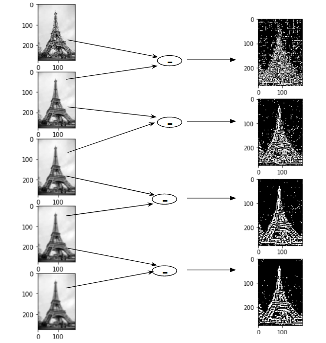
Here is an example making use of a picture of the Tour Eiffel . We have the original image of size $(275, 183)$ and a scaled image of dimension $(138, 92)$. For both the images, two blur images have been created.

To create the octave, we first need to choose the number of images we want in each octave. This is denoted by $s$. Then $\sigma$ for the Gaussian filter is chosen to be $2^(1/s)$. Since blur accumulates multiplicatively, when we blur the original image with this filter $s$ times, the result will have blur $= 2 \times$ original blur.

One detail from the Lowe's paper that is rarely seen mentioned is that in each octave, you actually need to produce $s+3$ images (including the original image). This is because when adjacent levels are subtracted to obtain the approximated LoG octave (i.e. the DoG), we will get one less image than in the Gaussian octave:

image from the original paper

Now we have $s+2$ images in the DoG octave. However, later when we look for extrema in the DoG, we will look for the min or max of a neighborhood specified by the current and adjacent levels. We will describe this later on, for the moment being, we have generated the Gaussian octave, we downsample the top level by two and use that as the bottom level for a new octave. The original paper uses four octaves.

To conclude this section, let us illustrate the situation in the Eiffel Tower example: a good set of octaves may be the following one

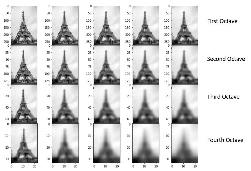
Note that each octave is a set of images sharing the same scale, we apply the DoG to images in the octave getting a version of images where we have feature enhancement.

The DoG result is the following

One can easily implement all of this by some python code. This is not the goal of this repository, so we refer to an excellent medium article for details.

Summary scheme

Here we collect the main points of the part one of the algorithm, that is the construction of scale-space or Gaussian pyramid.

Given the original image, apply the blur filter to add a double the blur $s$ times.
Half the scale of the image to create different octaves.
Apply the DoG to get the feature enhanced version of the octave.

Keypoint localisation

Once the scale space has been defined, we are ready to localise the keypoints to be used for feature matching. The idea is to identify extremal points (maxima and minima) for the feature enhanced images.

To be concrete, we split this in two steps:

Find the extrema
Remove low contrast keypoints (also known under the name of keypoint selection)

Extremal point scanning

We will not dig into details of extremisation algorithms to find maxima and minima. Conceptually, we explore the image space (i.e. pixel by pixel) and compare each point value with its neighbouring pixels.

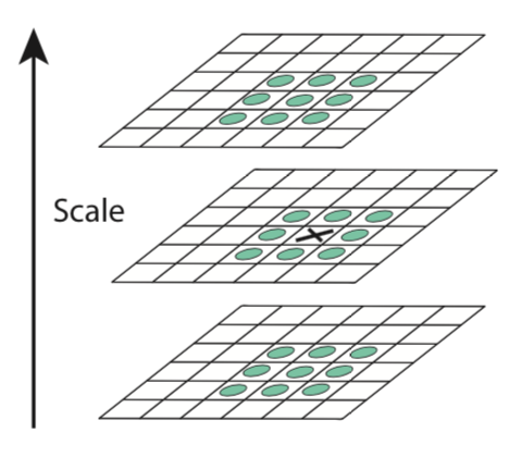
In other words, we scan over each scale-space DoG octave, $\mathcal{D}$, and include the center of each $3 \times 3 \times 3$ neighbourhood as a keypoint if it is the minimum or maximum value in neighbourhood.

This is the reason the algorithm has generated $s+2$ levels in the DoG octave. One cannot scan over the points in the top or bottom level, but one still wants to get keypoints over a full octave of blur.

Keypoints so selected are scale-invariant, however, they yield many poor choices and/or noisy, so in the next section we will throw out bad ones as well refine good ones.

Keypoint selection

The guide principle leading us to keypoint selection is

Let's eliminate the keypoints that have low contrast, or lie very close to the edge.

This because low-contrast points are not robust to noise, while keypoints on edges should be discarded because their orientation is ambiguous, thus they will spoil rotational invariance of feature descriptors.

The recipe to cook good keypoints goes through three steps:

Compute the subpixel location of each keypoint
Throw out that keypoint if it is scale-space value at the subpixel is below a threshold.
Eliminate keypoints on edges using the Hessian around each subpixel keypoint.

In many images, the resolution is not fine enough to find stable keypoints, i.e. in the same location in multiple images under multiple conditions. Therefore, one can perform a second-order Taylor expansion of the DoG octave to further localize each keypoint. Explicitly,

$$ \mathcal{D} = \mathcal{D} + \partial_x \mathcal{D}^T + \frac{1}{2} x^T \left(\partial^2_{x^2} \mathcal{D}\right) x , .$$

Here, $x$ is the three-dimensional vector $[x, y, \sigma]$ corresponding to the pixel location of the candidate keypoint. Taking the derivative of this equation with respect to $x$ and setting it equal to zero yields the subpixel offset for the keypoint,

$$ \bar{x} = - \left(\partial^2_{x^2} \mathcal{D}\right)^{-1} \partial_x \mathcal{D} , . $$

This offset is added to the original keypoint location to achieve subpixel accuracy.

At this stage, we have to deal with the low contrast keypoints. To evaluate if a given keypoint has low contrast, we perform again a Taylor expansion.

Remind we do not just have keypoints, but subpixel offsets. The subpixel keypoint contrast can be calculated as,

$$ \mathcal{D}(\bar{x}) = \mathcal{D} + \frac{1}{2}\partial_x\mathcal{D}^T \bar{x}, ,$$

which is the subpixel offset added to the pixel-level location. If the absolute value is below a fixed threshold, we reject the point. We do this because we want to be sure that extrema are effectively extreme.

Finally, as said we want to eliminate the contribution of the edge keypoints, because they will break rotational invariance of the descriptors. To do this, we use the Hessian calculated when computing the subpixel offset. This process is very similar to finding corners using a Harris corner detector.

The Hessian has the following form,

$$ \mathcal{H} = \begin{pmatrix} D_{xx} & D_{xy} \\ D_{yx}& D_{yy} \end{pmatrix} . $$

To detect whether a point is on the edge, we need to diagonalise, that is find eigenvalues and eigenvectors of such Hessian matrix. Roughly speaking and being schematic, if the eigenvalues of $\mathcal{H}$ are both large (with respect to some scale), the probability the point is on the edge is high. We refer again to the original paper.

Orientation assignement

Getting the keypoints is only half the battle. Now we have to obtain the actual descriptors. But before we do so, we need to ensure another type of invariance: rotational.

We have ensured translational invariance thanks to the convolution of our filters over the image. We also have scale invariance because of our use of the scale-normalized LoG filter. Now, to impose rotational invariance, we assign the patch around each keypoint an orientation corresponding to its dominant gradient direction.

To assign orientation, we take a patch around each keypoint thats size is proportional to the scale of that keypoint.

Consider the image below.

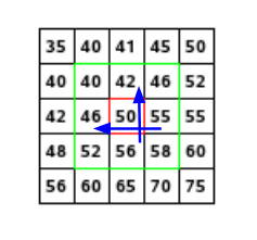
One can calculate the following quantities,

$$ r = \sqrt{\left(\partial_x f\right)^2 + \left(\partial_y f\right)^2} , \quad \phi = \mathrm{atan}{\left(\partial_x f / \partial_y f\right)} $$

called respectively magnitude and orientation. They are functions of the gradient in each point. To summarise, we can state

The magnitude represents the intensity of the pixel and the orientation gives the direction for the same.

We can now create a histogram given that we have calculated these magnitude and orientation values for the whole pixel space.

The histogram is created on orientation value (the gradient is specified in polar coordinates) and has 36 bins (each bin has a width of 10 degrees). When the magnitude and angle of the gradient at a pixel is calculated, the corresponding bin in our histogram grows by the gradient magnitude weighted by the Gaussian window. Once we have our histogram, we assign that keypoint the orientation of the maximal histogram bin.

To rephrase, let's look at the histogram below.

This histogram would peak at some point. The bin at which we see the peak will be the orientation for the keypoint. Additionally, if there is another significant peak (seen between 80 – 100%), then another keypoint is generated with the magnitude and scale the same as the keypoint used to generate the histogram. And the angle or orientation will be equal to the new bin that has the peak.

Effectively at this point, we can say that there can be a small increase in the number of keypoints.

Local descriptors

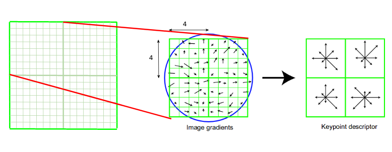
Finally we got at the final step of SIFT. The previous step gave us a set of stable keypoints, which are also scale-invariant and rotation-invariant. Now, we can create the local descriptors for each keypoint. We will make use of points in the neighbourhood of each keypoints to characterise it completely. The keypoint endowed with these local properties is called a descriptor.

A side effect of this procedure is that, since we use the surrounding pixels, the descriptors will be partially invariant to illumination or brightness of the images.

We will first take a $16 \times 16$ neighbourhood around the keypoint. This $16 \times 16$ block is further divided into $4 \times 4$ sub-blocks and for each of these sub-blocks, we generate an $8$-bin histogram using magnitude and orientation as described above. Finally, all of these histograms are concatenated into a $4\times 4 \times 8 =128$ element long feature vector.

This final feature vector is then normalized, thresholded, and renormalized to try and ensure invariance to minor lighting changes.

Each of these arrows represents the 8 bins and the length of the arrows define the magnitude. So, we will have a total of 128 bin values for every keypoint.

To finally summarise,

A local descriptor is a set of features, encoded by a feature vector, describing magnitude and orientation of neighbourhood for each keypoint.

The optimised version: Speeded Up Robust Feature

Getting dirty: examples

Easy task: Compare two coins

A not-so-easy task: Compare two radiographs

Metric: a score to quantify how similar are two images

The aim of this section is to define a metric to measure the amount of similarity of two images. Actually, what we want to measure is the degree of confidence of a match between two images.

In order to define such a metric, we can fix some key properties any good metric must satisfy.

It has to be positive-defined, i.e. $g(\gamma_1, \gamma_2) \geq 0$, $\forall \gamma_1, \gamma_2$.
The metric calculated on the same image has to be equal to one, i.e. $g(\gamma, \gamma) =1$, $\forall \gamma$

Conclusions and further developments

Acknowledgements

I would like to acknowledge both openCV and menpo projects.

The descriptive sections refers to different sources like Wikipedia, Scholarpedia, medium articles and the original papers and one may find further details there.
SIFT algorithm was patented in Canada by the University of British Columbia and published by David Lowe in 1999.

oscar-defelice/teeth-recognition