Pattern Recognition Course Assignment 1: Face Recognition
Authors: Amr Elzawawy & Omar Swidan at March 2019
Introduction
Face recognition has become a major field of interest these days. Face recognition algorithms are used in a wide range of applications such as security control,crime investigation, and entrance control in buildings, access control at automatic teller machines, passport verification, identifying the faces in a given databases. Formally, Face recognition is the bio-metric identification by scanning a person’s face and matching it against a library of known faces. In this assignment, we implement two different image recognition approaches. The first is Eigenfaces which is one of the most widely used representations, which are based on principal component analysis and use a nearest neighbour classifier. The second is Fisherfaces which use linear/Fisher discriminant analysis (FLD/LDA) for best discriminating the face images of same class and also use a nearest neighbour classifier.
Approach one: Classification using Eigenfaces and Principal component analysis
PCA is also known as Karhunen Loeve projection.Principal component analy- sis (PCA) is a statistical procedure that uses an orthogonal transformation to convert a set of observations of possibly correlated variables (entities each of which takes on various numerical values) into a set of values of linearly uncor- related variables called principal components and refrred to as Eigenfaces. In PCA, the main idea to re-express the available dataset to extract the relevant information by reducing the redundancy and minimize the noise. A nearest neighbour classifier works afterwards by comparing compare a face’s position in Eigenfaces subspace with the position of known individuals and the distances between them.
Algorithm
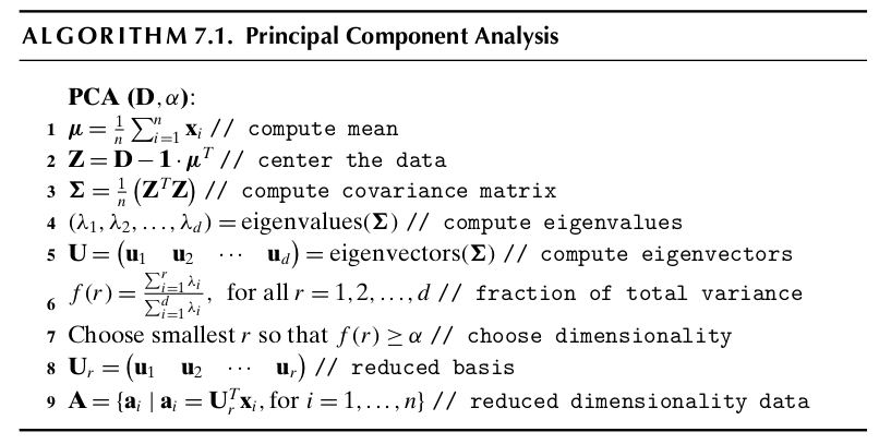
PCA algorithm steps and procedure is provided in Figure 1 which is taken from [1] from Chapter 7.
PCA is mathematically defined as an orthogonal linear transformation that transforms the data to a new coordinate system such that the greatest variance by some projection of the data comes to lie on the first coordinate (called the first principal component), the second greatest variance on the second coordinate, and so on. PCA calculates the Eigenvectors of the co-variance matrix, and projects the original data onto a lower dimensional feature subspace, which is defined by Eigenvectors with large Eigenvalues. The coordinates of the data points in the lower subspace dimension is computed and fed to the classifier after this algorithm job ends.
Implementation and Results.
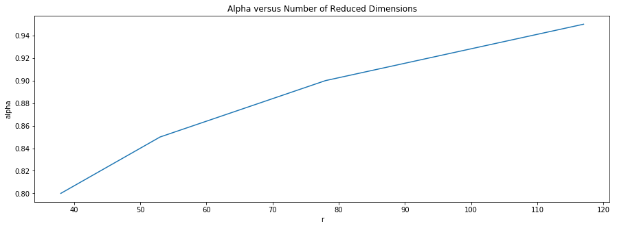
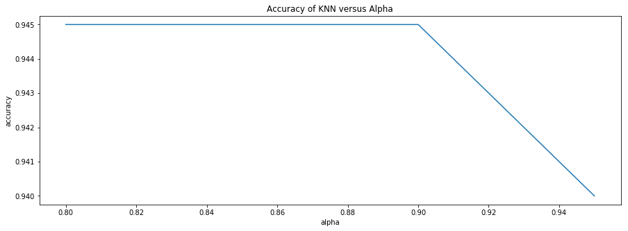
We implemented the above algorithm in Figure 1 using Python and Numpy arrays. The results shown in this section are related to the 50-50 data split test, results on the 70-30 data split test can be obtained from the source code attached and referred to later on. Computing the mean vectors of each dimen- sion, normalizing the data, and computing the co-variance matrix, Eigenvalues and Eigenvectors. After Projection of data, we obtain the coordinates A matrix and use finally the simple (i.e k = 1) k-nearest neighbour classifier to determine the class labels of testing data. We established four trials when choosing the di- mensionrbased on four different values ofα: 0.8 , 0.85, 0.9, 0.95 which yielded different values ofrand recomputed the accuracy of the classifier for each trial. Figures 2 and 3 show a plot of the relation betweenrandαand betweenαand accuracy of the KNN classifier respectively. From figure 2, it can be deduced
that as alpha increases, the number of reduced dimensions required to achieve that alpha value increases. It is then obvious from figure 3, that after a certain alpha value there is no clear or big change in accuracy and it actually decreases when alpha is set to 0.95 as it is over-fits. So, we can deduce the best alpha value here is 0.8, which achieves very good accuracy with no or little redundant dimensions in the subspace.
Visualization of EigenFaces
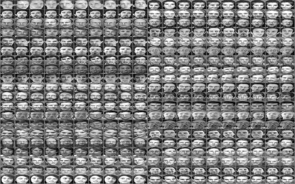
The aim of this section is to better grasp the concept of Eigenfaces in action rather than in mathematical formulas and codes. First,the dataset we worked on in this assignment is the ATT face database (formerly the ORL database)[2]. It is heavily used in publications as an example of an easy set of images as the pictures are taken under very similar conditions. There are ten different images of each of 40 distinct classes(i.e persons). For some subjects, the images were taken at different times, varying the lighting, facial expressions (open / closed eyes, smiling / not smiling) and facial details (glasses / no glasses). All the images were taken against a dark homogeneous
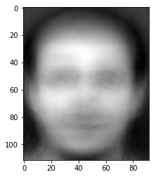
background with the subjects in an upright, frontal position (with tolerance for some side movement). A preview image of the Database of Faces is shown in Figure 4. Second, we split the photos into training and test sets using two different splits in two different files ( 50-50 splits and 70-30 splits). The mean face is the face that resembles roughly most of the dataset faces features, the mean face of the train set, in case of 50-50 is shown in Figure 5.
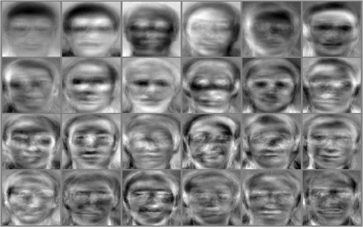
Then, we completed the procedure as explained in 2.2 and the Eigenfaces
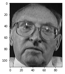
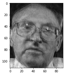
produced as those shown in Figure 6. Finally, to complete the purpose of this section, we show the reconstruction of a sample face via the Eigenfaces obtained. Figure 7(a) shows the original face while 7(b) shows the reconstructed one.
So, to summarize our work in the first approach, Eigenfaces along with a simple KNN Classifier did a very good job in faces classification as well as face reconstruction experiment conducted on a sample test face.
Approach two: classification using Linear Discriminant Analysis
Linear discriminant analysis (LDA), also called normal discriminant analysis (NDA), or discriminant function analysis is a generalization of Fisher’s linear discriminant, a method used in statistics, pattern recognition and machine learn- ing to find a linear combination of features that characterizes or separates two or more classes of objects or events. Ronald A. Fisher formulated the Linear Discriminant in 1936 in [3], and it also has some practical uses as classifier. The original Linear discriminant was de- scribed for a 2-class problem, and it was then later generalized as “multi-class Linear Discriminant Analysis” in [4]. The goal of LDA is to project a feature space (a dataset n-dimensional samples) onto a smaller subspace k (where k is smaller than or equal to n-1) while main- taining the class-discriminatory information. In other words, it seeks to reduce dimensionality while class separation in mind.
Algorithm
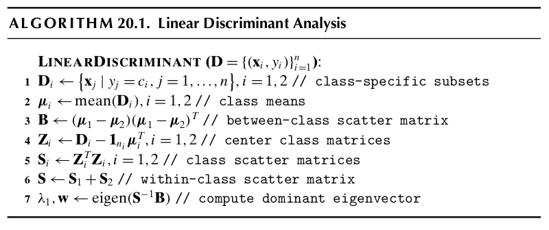
LDA algorithm steps and procedure is provided in Figure 8 which is taken from [1] from Chapter 20.
As the algorithm lists, the steps involved in the algorithm is as follows. Step one, compute d-dimensional mean vectors for different classes from the dataset, where d is the dimension of feature space.Step two, compute in-between class and with-in class scatter matrices.Step three, compute Eigenvectors and corre- sponding Eigenvalues for the scatter matrices. Step four, choose k Eigenvectors corresponding to top k Eigenvalues to form a transformation matrix of dimension dxk. Step five, transform the d-dimensional feature space X to k-dimensional feature subspace Y via the transformation matrix.
Implementation and results
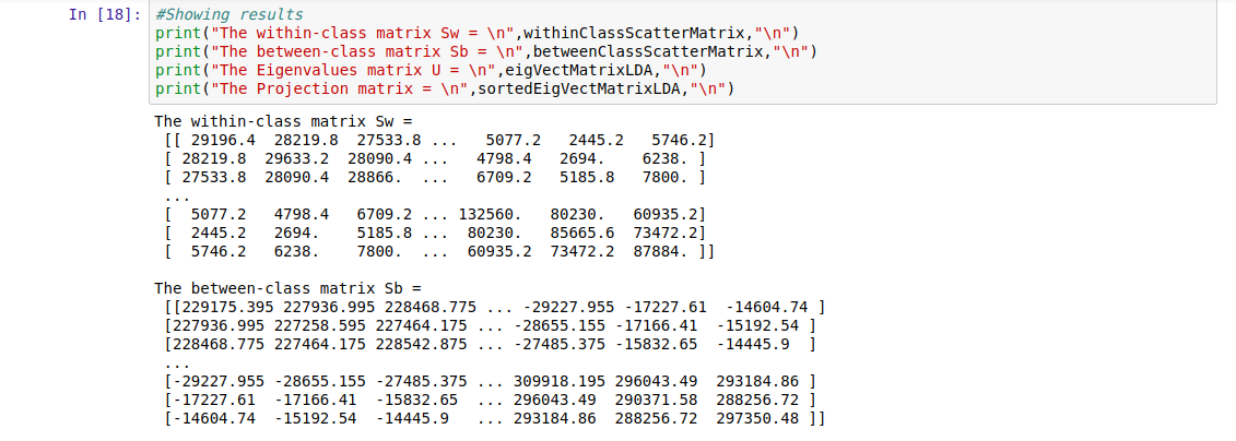
Again, we implemented the above algorithm in Figure 8 using Python and Numpy arrays. In order to find a good projection vector, we need to define a measure of separation between the projections. However, the distance between the projected means is not a very good measure since it does not take into account the standard deviation within the classes. The solution proposed by Fisher is to maximize a function that represents the difference between the means, normalized by a measure of the within-class variability, or the so-called scatter.The Fisher linear discriminant is defined as the linear functionwTxthat maximizes the criterion function: (the distance between the projected means normalized by the within-class scatter of the projected samples. Therefore, we will be looking for a projection where examples from the same class are projected very close to each other and, at the same time, the projected means are as farther apart as possible. Thus, It can be shown that the optimal projection matrix W∗is the one whose columns are the eigenvectors corresponding to the largest eigenvalues of generalized eigenvalue problem. The main resulting matrices of the implementation is shown in figures below, more can be found in the source code though.
Finally, we note the KNN classifier scores using LDA on (50-50) and (70-30) splits were 0.55 and 0.64 respectively.
Limitations of LDA
Although, LDA sounds fancy and a good option it is wise to consider it’s prob- lems and whether it is going to be a good choice for you when applying it on your data or not. Firstly, LDA produces at most C-1 feature projections. If the classification error estimates establish that more features are needed, some other method must be employed to provide those additional features. Secondly,LDA is a parametric method since it assumes uni-modal Gaussian like- lihoods. If the distributions are significantly non-Gaussian, the LDA projections will not be able to preserve any complex structure of the data, which may be needed for classification. Lastly, LDA will fail when the discriminatory information is not in the mean but rather in the variance of the data.
In any of these cases do occur, you can consider other variants of LDA that solve some of those limitations mentioned above such as Non-parametric LDA, Orthonormal LDA , Generalized LDA and Multilayer perceptrons. Moreover, you can be directed otherwise to use a totally different dimension reduction technique such as PCA, Exploratory Projection Pursuit or Sammon’s non-linear mapping.
Conclusion
In general, dimensionality reduction does not only help reducing computational costs for a given classification task, but it can also be helpful to avoid over-fitting by minimizing the error in parameter estimation (“curse of dimensionality”). In this work, we worked in the aim to implement a face recognition software based
on KNN Classification and using dimensionality reduction before applying it to the classifier with two approaches, one was LDA and the other was PCA.
PCA vs LDA
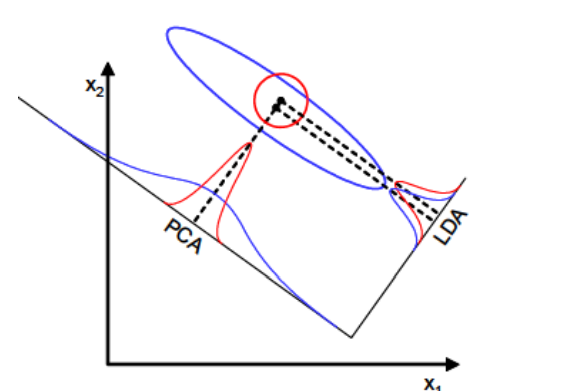
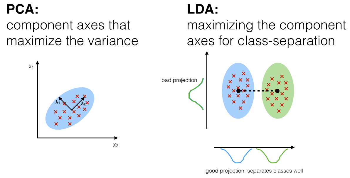
LDA is also closely related to principal component analysis (PCA) and in that they both look for linear combinations of variables which best explain the data.LDA explicitly attempts to model the difference between the classes of data. PCA on the other hand does not take into account any difference in class, and factor analysis builds the feature combinations based on differences rather than similarities.
Both Linear Discriminant Analysis (LDA) and Principal Component Anal- ysis (PCA) are linear transformation techniques that are commonly used for di- mensionality reduction. PCA can be described as an “unsupervised” algorithm, since it “ignores” class labels and its goal is to find the directions (the so-called principal components) that maximize the variance in a dataset. In contrast to PCA, LDA is “supervised” and computes the directions (“linear discriminant”) that will represent the axes that that maximize the separation between multiple classes. Although it might sound intuitive that LDA is superior to PCA for a multi-class classification task where the class labels are known, this might not always the case. For example, comparisons between classification accuracies for image recognition after using PCA or LDA show that PCA tends to outperform LDA if the number of samples per class is relatively small as shown in [5]. In practice, it is also common to use both LDA and PCA in combination: E.g., PCA for dimensionality reduction followed by an LDA, this approach is called the Fisher Faces and was proposed in [6]. As we mention later on, one of our
future improvement tasks is to implement this approach and compare it with our work here. Also in case of uniformly distributed data, LDA almost always performs better than PCA. However if the data is highly skewed (irregularly distributed) then it is advised to use PCA since LDA can be biased towards the majority class.
Future Improvements and Goals
In this section we would like to point out some final notes that we would like to do futuristic improvements in our source code and implementation. One of those being is implementing the Fisher Faces approach (Applying PCA first then feeding it as input to the LDA) and comparing it with the two approaches already implemented in order to get a full view of the idea. Also, we would like to apply some OOP and modularity in our code by breaking down the source code into various python files in which there is a Utility class for the helper methods and also a main class for the ML algorithms applied. Also, it is important to point out that the accuracy scores achieved by LDA was unsatisfactory like those obtained from PCA so maybe a last goal is to ensure that our implementations are correct and that this is just the nature’s work.
References
[1]Data Mining and Analysis: Fundamental Concepts and Algorithms MO- HAMMED J. ZAKI Rensselaer Polytechnic Institute, Troy, New York WAG- NER MEIRA JR. Universidade Federal de Minas Gerais, Brazil
[2]ATT Face database, or formally ORL Faces
[3]”The Use of Multiple Measurements in Taxonomic Problems” by Ronald A. Fisher in 1936
[4]”Multiple Discriminant Analysis” by C. R. Rao in 1948
[5]PCA vs. LDA, A.M. Martinez et al., 2001
[6]”Eigenfaces vs. Fisherfaces: Recognition Using Class Specific Linear Pro- jection” by Peter N. Belhumeur, Joao P. Hespanha, and David J. Kriegman
[7]FACE RECOGNITION USING PCA, LDA AND VARIOUS DISTANCE CLASSIFIERS
