Simulating Molecular Dynamics with Large Timesteps using Recurrent Neural Networks

JCS Kadupitiya, Geoffrey C. Fox, Vikram Jadhao | 2020

Molecular dynamics simulations rely on numerical integrators such as Verlet to solve the Newton's equations of motion. Using a sufficiently small timestep to avoid discretization errors, Verlet integrators generate a trajectory of particle positions as solutions to the equations of motions. We introduce an integrator based on recurrent neural networks that is trained on trajectories generated using Verlet integrator and learns to propagate the dynamics of particles with timestep up to 4000 times larger compared to the Verlet timestep. We demonstrate significant net speedup of up to 32000 for few-particle (1 - 16) 3D systems and over a variety of force fields.
Paper: https://arxiv.org/abs/2004.06493
Cite as:

@misc{kadupitiya2020simulating,
    title={Simulating Molecular Dynamics with Large Timesteps using Recurrent Neural Networks},
    author={JCS Kadupitiya and Geoffrey C. Fox and Vikram Jadhao},
    year={2020},
    eprint={2004.06493},
    archivePrefix={arXiv},
    primaryClass={physics.comp-ph}
}

Directory Structure

.
├── data                 # All the datafiles for experiments are here, read the readme inside
├── figures              # Main fugures are here
├── models               # Pretrained LSTM models are here
├── paper                # latex files for the paper
├── scripts              # Supporting python scripts for MD-visualization
└── src                  # Codes needed to run RNN-MD
    ├── config           # All the configurations for RNN models are in YAML files
    ├── md-codes         # MD codes in python and c++
    ├── model            # Main codebase for RNN-MD
    ├── paper-figures    # Python notebooks used to generate the figures for the paper
    ├── spec.._local     # Python notebook version of the RNN-MD 
    ├── spec.._colab     # google colab notebook version of the RNN-MD 
    ├── temp_data        # temporary data folders for visualization
    ├── DW-Ex..ipynb     # Double well experiment
    ├── LJ-Ex..ipynb     # Lennord Jones experiment
    ├── Ru.-Ex..ipynb    # Rugged potential experiment
    ├── SHO-Ex..ipynb    # SHO experiment        
    ├── Ma.-Ex..ipynb    # Many particle PB experiment

Note: We encourage the use of notebooks at source level (src) compared to the notebooks at src/spec...
- This is because the notebooks at the src level demonstrate how to use the model with src/model code which uses one code base for all the experiments with different configuration files (src/config).
- On the other hand, the notebooks which are at src/spec.., are standalone notebook versions of src/model.
- The following example explains the use of ource level (src) notebooks as it is much easier to understand.

Example Model Training and Testing

First, git clone the project: git clone https://github.com/softmaterialslab/RNN-MD.git
Next, go to src directory and run the following in a python 3 environment.
If you want to change any configuration, please edit the src/config/SHO.yaml file.
Then, load the module and load configuration from SHO.yaml file.

from model.RNN_MD import RNN_MD
rnn_md = RNN_MD(experiment='sho')

Next, load dataset: rnn_md.load_data()
Then, train and save the model:

rnn_md.train()
rnn_md.save_model()

Similary, if you have a pretrained model in model directory, load it as follows: rnn_md.load_model()
Then use the model to run a RNN-MD simulation:

import matplotlib.pyplot as plt
%matplotlib inline

rnn_md.simulate_new(testing_index=1)

fig=plt.figure(figsize=(16, 6))
plt.title(rnn_md.input_list[rnn_md.sim_])
plt.plot(rnn_md.actual_output,'r+', label='MD_dynamics', linewidth=1, markersize=3, linestyle='dashed')
plt.plot(rnn_md.predicted_output, label='MD-RNN')
plt.plot(rnn_md.Only_RNN_predicted_output, label='continous RNN')
plt.legend()

All the experiments canbe run using similar setup, please check notebooks available in src directory.

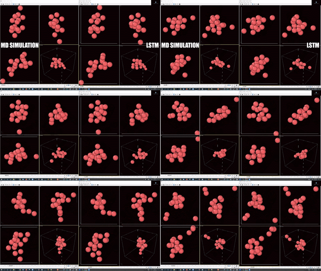
Example results for 16 particle periodic boundry simulation

Example simulations with LJ potentail, 16 particle in a periodic boundary simulation:

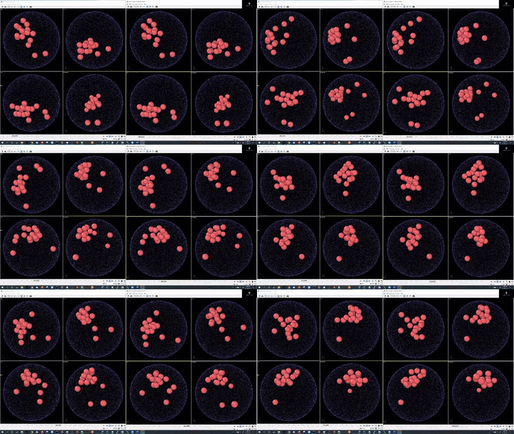
Example simulations with LJ potentail, 16 particle in a spherical hard wall simulation:

Architecture Figures

Overview of the deep learning approach:

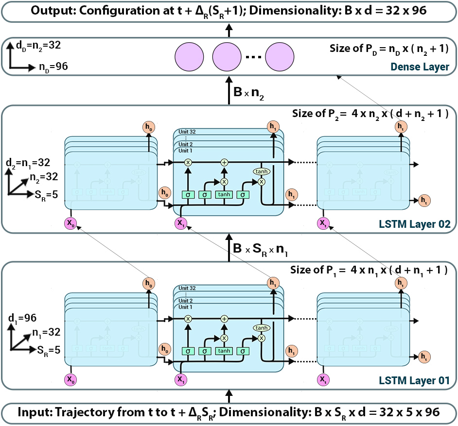
RNN-MD architecture:

owaisahmad18/RNN-MD

Simulating Molecular Dynamics with Large Timesteps using Recurrent Neural Networks

Directory Structure

Example Model Training and Testing

Example results for 16 particle periodic boundry simulation

Architecture Figures