This code implements the EM algorithm to fit the Mixture of Gaussians with different models in MATLAB. A sample data is given to work on. This data set consists of three classes of 1000 observations each. Each observation has two features. The data file includes the observations as rows, the features as the first and second columns, and the class label for each observation as the third column. In the code, class1 corresponds to 'blue', class2 corresponds to 'red' and class3 corresponds to 'green' samples. Each class is divided into two sets and one half is used for training and the other half for testing.
In order to start to process, it is enough to run the "run.m". There are some parameters to determine the number of Gaussians and the iteration amount for Expectation-Maximization. After setting the parameters, the algorithm runs for spherical, diagonal and arbitrary covariance matrices of Gaussians. The kind of a covariance matrix is determined in "EM.m" function with the "gaussCase" parameter.
Before the main process, mixing parameter(alpha) mu and sigma values are initialized. Mu is initialized with the cluster center of k-means algorithm. Sigma is initialized as an identiy matrix in 2x2 dimension. Mixing parameter (alpha) is initialized as 1/componentNumber since sum of mixture parameters should equal to "1".
After initializing all parameters, EM algorithm is starting. EM, updates mu ,sigma and mixing parameter(alpha) at each iteration in order to fix the mixtures on data. So, it finds final mixture models for classification. In the code, iteration stops according to log-likelihood. EM algorithm tries to maximize likelihood. Therefore, if log-likelihood that calculated at previous iteration is not necessarily different than the current log-likelihood, EM iteration should stop. Here is the log-likelihood formula:

Therefore, after calculating the p(x|μ, Σ), log-likelihood is estimated and according to that value updating process is pursued. In update part, each component's parameters such as mu, sigma and mixing parameter(alpha) are updated according to given formulas below. While calculating p(x|μ, Σ), MATLAB's mvnpdf function is used.
- Update alpha:

where,

- Update mu:

- Update covariance matrix for model 1 (Spherical):
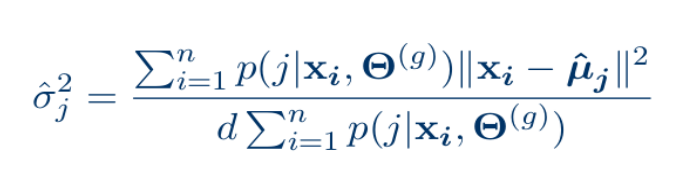
- Update covariance matrix for model 2 (Diagonal):

- Update covariance matrix for model 1 (Arbitrary):

Here is some results where component number = 5 and iteration number = 100.
- For model 1 (Spherical Gaussian):

- For model 2 (Diagonal Gaussian):

- For model 3 (Arbitrary Gaussian):
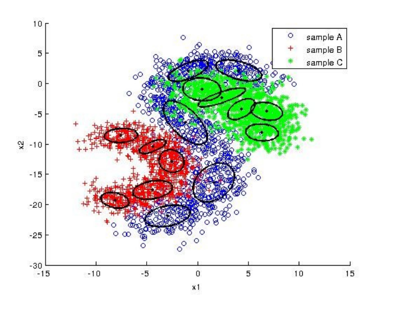
According to graphs, we can say that the best fitted model is arbitrary Gaussian model since it is flexible. Therefore, it fits to data better and the classifier gives more accurate results.