- ihydro
- 1 Introduction
- 2 System setup and installation
- 3 Prepare DEM
and Sampling Points for analysis
- 3.1 Generate toy terrain dataset and sampling points
- 3.2
Generate flow direction/accumulation geospatial analysis products with
process_flowdir() - 3.3
Generate vector geospatial analysis products with
generate_vectors() - 3.4
Create lookup tables of flow-directions with
trace_flowpaths() - 3.5
Generate complete upstream catchment areas with
get_catchment() - 3.6 Generate entire hydrology workflow in one step.
- 4 Examining Pairwise Instream Distances
- 5 Process layers of interest
- 6 Calculate (weighted) spatial summaries:
- 7 Example Modelling
- 8 Future Plans
- 9 References
Aquatic environmental scientists are often interested in relating landscape features to observed responses (e.g., fish size, water temperature, invertebrate community composition, etc.) in streams, rivers and lakes. The computational workflow for conducting these investigations is complex. Simply describing how water flows and accumulates across the landscape can be a challenge itself, but for aquatic scientists it is only the first step. The stream network must then be extracted from the landscape, and reaches (a.k.a. segments; i.e., stretches of river between two confluences) identified and given unique identifiers. These reaches must then be attributed to be informative (e.g., slope, stream order, upstream channel length, etc.); and upstream-downstream connectivity between reaches established.
Typically, observed responses are measured at discrete sampling locations along the stream network. If the location information is to be preserved (i.e., if samples are upstream and downstream of a particular effluent outflow), they must be incorporated into the network. This is done by splitting stream lines and catchments at these points.
Once that is done, landscape features of interest (e.g., land-cover, geology, climate, etc.) must be related to the reach (or sampling points). This alone can be complex as the spatial configuration of these factors relative to flow direction and accumulation can be important (Peterson et al., 2011). The ihydro package uses hydroweight (Kielstra et al. 2021) to calculate these attributes.
The complexity of this workflow can be a rate limiting step in the scope, content, quality, and applicability of investigations by aquatic environmental scientists. The ihydro package offers tools and workflows to simplify these complex steps. It is capable of handling all above computation steps, leaving researchers the task of identifying layers of interest and modeling with (potentially) large numbers of predictors.
The ihydro package also implements descriptions of spatial autocorrelation among sites. Due to the linear nature of flow in streams and rivers, autocorrelation tends to be asymmetric, with sites generally more similar when they are flow connected, than not flow connected. ihydro produces tables that can be transformed into an asymmetric matrices that describes the relationships between sampling points based on instream distances and/or the proportions shared catchments. Proportion of shared upstream catchment (rather than in-stream distance) are a more relevant measure of spatial autocorrelation in streams because it accounts for differences in catchment areas between points, as well as spatial proximity. For example, if water chemistry samples are taken from a large 6th order stream, and a upstream small 1st order tributary we would expect the small tributary to have only a small impact on the larger stream (despite its close physical proximity). Hence, autocorrelation should be low because the tributary does not contribute much flow to the larger stream. Using in-stream distances alone may misrepresent this pattern.
ihydro stores its geospatial products in a geopackage file for ease of retrieval and extraction in external software (i.e. QGIS). Many ihydro functions can be run in parallel for increased speed (if enough memory is available). The functions are also quick at removing internal intermediate files to keep hard drives from filling up too fast.
WhiteboxTools and whitebox are required for ihydro. See whiteboxR or below for installation.
## Follow instructions for whitebox installation accordingly
## devtools::install_github("giswqs/whiteboxR") # For development version
## whitebox is now available on CRAN
#install.packages("whitebox")

library(whitebox)

if (F){
  install_whitebox()
  # Possible warning message:
  # ------------------------------------------------------------------------
  # Could not find WhiteboxTools!
  # ------------------------------------------------------------------------
  #
  # Your next step is to download and install the WhiteboxTools binary:
  #     > whitebox::install_whitebox()
  #
  # If you have WhiteboxTools installed already run `wbt_init(exe_path=...)`':
  #    > wbt_init(exe_path='/home/user/path/to/whitebox_tools')
  #
  # For whitebox package documentation, ask for help:
  #    > ??whitebox
  #
  # For more information visit https://giswqs.github.io/whiteboxR/
  #
  # ------------------------------------------------------------------------
}Begin by bringing in the digital elevation model.
## Load libraries
# remotes::install_github("p-schaefer/ihydro)
library(ihydro)
library(tmap)
library(furrr)
library(whitebox)
library(terra)
library(sf)
library(dplyr)
library(tidyr)
library(purrr)

# Many function in 'ihydro' can be run in parallel internally.

# Parallelization is done through the future package, so all parallel backends
# should be supported i.e.,:
plan(multisession(workers=4))

## Generate save_dir as a temporary directory
save_dir <- tempdir()


## Import toy_dem from openSTARS package
# devtools::install_github("MiKatt/openSTARS", ref = "dev")

ot<-system.file("extdata", "nc", "elev_ned_30m.tif", package = "openSTARS") %>%
  rast()

crs(ot)<-crs(rast(system.file("extdata", "nc", "landuse_r.tif", package = "openSTARS")))
writeRaster(ot,file.path(save_dir, "toy_dem.tif"),overwrite=T)

toy_dem<-rast(file.path(save_dir, "toy_dem.tif"))

## Identify some sampling points
system.file("extdata", "nc", "sites_nc.shp", package = "openSTARS") %>%
  vect() %>%
  st_as_sf() %>%
  st_transform(st_crs(toy_dem)) %>%
  vect() %>%
  writeVector(file.path(save_dir, "sites.shp"),overwrite=T)

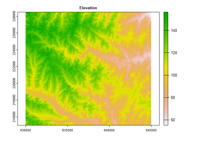
plot(toy_dem,main="Elevation")The DEM must be processed in a way to remove depressions. Whitebox
offers methods for breaching and filling DEMs to remove depressions.
These may be applied before had, or through the depression_corr
argument in process_flowdir().
Another factor to consider at this step is whether to burn a stream
vector into the DEM; ihydro implements a simplified stream burning
method that lowers the evation along the DEM by burn_depth meters. See
here
for more detailed approaches.
# Outputs of all functions are always saved to output_filename by default,
# but can be included in function return with return_products=T (note this can
# be very slow for large regions)
output_filename_hydro<-file.path(save_dir,"Processed_Hydrology.gpkg")

# Generates d8 flow direction and accumulation, extracts streams at a specified
# flow accumulation threshold
hydro_out<-process_flowdir(
  dem=toy_dem,
  burn_streams=system.file("extdata", "nc", "streams.shp", package = "openSTARS"),
  burn_depth=5,
  min_length=3,
  depression_corr="breach",
  threshold=100L,
  return_products=T,
  output_filename=output_filename_hydro,
  temp_dir=NULL,
  verbose=T
)

# List files present in gpkg
ihydro_layers(hydro_out)
#> # A tibble: 7 × 3
#>   layer_name       data_type data_group
#>   <chr>            <chr>     <chr>
#> 1 dem_final        Raster    hydro
#> 2 dem_d8           Raster    hydro
#> 3 dem_accum_d8     Raster    hydro
#> 4 dem_accum_d8_sca Raster    hydro
#> 5 dem_streams_d8   Raster    hydro
#> 6 DEM_Extent       Table     meta
#> 7 DEM_Extent       Vector    meta

# hydro_out$outfile # -> This is the full file path of the resulting geopackage (gpkg) file

# remaining outputs only present when `return_products` == T
# hydro_out$dem_final.tif # -> final dem after stream burning and depression correction
# hydro_out$dem_d8.tif # -> d8 flow direction
# hydro_out$dem_accum_d8.tif # -> d8 flow accumulation (cells)
# hydro_out$dem_accum_d8_sca.tif # -> d8 flow accumulation (specific catchment areas)
# hydro_out$dem_streams_d8.tif # -> extracted streams at specified `threshold`

# if `return_products` == F, all produces are only available in the gpkg file.
# terra and sf allow access to files directly in the gpkg file, whitebox
# requires them to be extracted to a folder

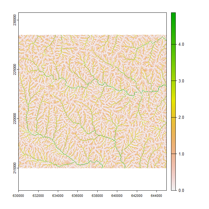
flow_accum<-rast(hydro_out$outfile,"dem_accum_d8")

plot(log10(flow_accum))
To create an ihydro object from an existing geopackage (i.e., created from a previous R run):
hydro_out_new<-as.ihydro(output_filename_hydro)
ihydro_layers(hydro_out_new)
#> # A tibble: 7 × 3
#>   layer_name       data_type data_group
#>   <chr>            <chr>     <chr>
#> 1 dem_final        Raster    hydro
#> 2 dem_d8           Raster    hydro
#> 3 dem_accum_d8     Raster    hydro
#> 4 dem_accum_d8_sca Raster    hydro
#> 5 dem_streams_d8   Raster    hydro
#> 6 DEM_Extent       Table     meta
#> 7 DEM_Extent Vector metaThis function combines generate_subbasins() and attrib_streamline()
to produce subcatchment polygons, stream lines, stream links (downstream
most points along each subcatchment), stream points (stream line
represented as individual points).
Typically, observed responses are measured at discrete sampling locations along the stream network. If the location information is to be preserved (i.e., if samples are upstream and downstream of a particular effluent outflow), the sampling points must be incorporated into the network. This is done by splitting stream lines and subcatchments at these points.
hydro_out<-generate_vectors(
  input=hydro_out,
  points=file.path(save_dir, "sites.shp"), # These are optional sampling locations
  site_id_col="site_id", # Column name in points layer that corresponds to
  #                      # unique IDs that will be available in data products
  snap_distance=100L, # points that are more than 100m from closest stream are excluded
  break_on_noSnap =F, # default is to stop when any points don't snap, this will ignore that
  return_products=T,
  temp_dir=NULL,
  verbose=T
)

ihydro_layers(hydro_out)
#> # A tibble: 22 × 3
#>    layer_name        data_type data_group
#>    <chr>             <chr>     <chr>
#>  1 dem_final         Raster    hydro
#>  2 dem_d8            Raster    hydro
#>  3 dem_accum_d8      Raster    hydro
#>  4 dem_accum_d8_sca  Raster    hydro
#>  5 dem_streams_d8    Raster    hydro
#>  6 Subbasins_poly    Table     hydro
#>  7 stream_lines      Table     hydro
#>  8 stream_links      Table     hydro
#>  9 stream_links_attr Table     hydro
#> 10 stream_points     Table     hydro
#> # … with 12 more rows

# Several important columns are used throughout the vector layers:
# `link_id` - identifies reaches/segments (stream length between two confluences)
# `trib_id` - identifies streams/tributaries, with the shortest channel getting
#           # a new trib_id at a confluence, and longest channel retaining the original ID
# `uslink_id` and `dslink_id`  - columns identify upstream and downstream links
# `ustrib_id` and `dstrib_id`  - columns identify upstream and downstream tributaries (longest
#  continuous flow-paths)

# If 'points' are provided, this function modifies the vector outputs by inserting
# links, and splitting lines/subbasins at `points`. Inserted points are given "link_id'
# values that increment with decimal places from downstream to upstream directions
# (i.e., 10.0 remains the pour point for the segment, and 10.1, 10.2,... identify
# sample points in an upstream direction).

# New layers added by `generate_vectors()`
# hydro_out$subbasins      # -> polygon subbasins attributed with `link_id` and reach
#                          #  contributing area (in m^2)
# hydro_out$stream_lines   # -> line vectors attributed with `link_id`
# hydro_out$points         # -> point vectors along lines identifying 'nodes' (confluence
#                          #  points), vs 'links' segments joining 'nodes', and also
#                          #  attributed with `link_id`, `trib_id`, upstream
#                          #  and downstream link and trib IDS and a number of extra attributes
# hydro_out$links          # -> point vector representing pour-points for subbasins,
#                          #  attributed with `link_id` and extra attributes
# hydro_out$snapped_points # -> provided points snapped to nearest segment. Any points
#                          #  beyond snap distance are removed, with a warning if
#                          #  break_on_noSnap == F.

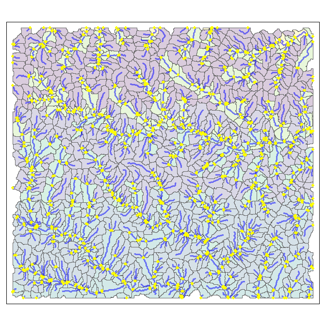
tm_shape(hydro_out$subbasins) + tm_polygons(col="link_id",palette = "viridis",alpha =0.2,legend.show=F) +
  tm_shape(hydro_out$stream_lines) + tm_lines(col="blue",alpha =0.5,legend.show=F,lwd =3) +
  tm_shape(hydro_out$links) + tm_dots(col="yellow",legend.show=F,size=0.15,border.col="black",border.alpha=1)
# Optional step, inserts sampling points into stream vectors, splitting subbasins
# and lines at sampling points, additional links inserted at sampling points as well
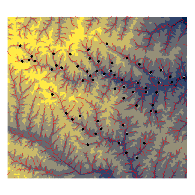
tm_shape(rast(hydro_out$dem_final.tif)) + tm_raster(palette = "cividis",legend.show=F) +
tm_shape(hydro_out$stream_lines) + tm_lines(col="red",alpha =0.5,legend.show=F,lwd =2) +
tm_shape(hydro_out$snapped_points %>% mutate(site_id=as.numeric(site_id))) +
tm_dots(col="darkgray",legend.show=F,size=0.35,border.col="black",border.alpha=1,border.lwd=1) +
tm_shape(read_sf(file.path(save_dir, "sites.shp"))) +
tm_dots(col="black",legend.show=F,size=0.35,border.col="black",border.alpha=1,border.lwd=1)To more efficiently generate catchments, look-ups are created that identify all upstream and downstream links originating from each link.
hydro_out<-trace_flowpaths(
  input=hydro_out,
  return_products=T,
  pwise_dist=T, # This will calculate all downstream flow-connected pairwise distances
  pwise_all_links=F, # This will calculate all flow un-connected pairwise distances (can be very time consuming)
  temp_dir=NULL,
  verbose=T
)

ihydro_layers(hydro_out)
#> # A tibble: 25 × 3
#>    layer_name       data_type data_group
#>    <chr>            <chr>     <chr>
#>  1 dem_final        Raster    hydro
#>  2 dem_d8           Raster    hydro
#>  3 dem_accum_d8     Raster    hydro
#>  4 dem_accum_d8_sca Raster    hydro
#>  5 dem_streams_d8   Raster    hydro
#>  6 ds_flowpaths     Table     flow_path
#>  7 us_flowpaths     Table     flow_path
#>  8 Subbasins_poly   Table     hydro
#>  9 stream_lines     Table     hydro
#> 10 stream_links     Table     hydro
#> # … with 15 more rows

# We will add these upstream and downstream lookup tables to the output below
con <- DBI::dbConnect(RSQLite::SQLite(), hydro_out$outfile)

hydro_out$us_flowpaths <-collect(tbl(con,"us_flowpaths"))
hydro_out$ds_flowpaths <-collect(tbl(con,"ds_flowpaths"))

DBI::dbDisconnect(con)

head(hydro_out$us_flowpaths)
#> # A tibble: 6 × 2
#>   pour_point_id origin_link_id
#>   <chr>         <chr>
#> 1 1             1
#> 2 10            10
#> 3 100           100
#> 4 1000          1000
#> 5 1000          1001
#> 6 1000          1004

head(hydro_out$ds_flowpaths %>% arrange(destination_link_id))
#> # A tibble: 6 × 2
#>   destination_link_id origin_link_id
#>   <chr>               <chr>
#> 1 1                   1
#> 2 10                  10
#> 3 100                 100
#> 4 1000                127
#> 5 1000                1107.1
#> 6 1000                1107

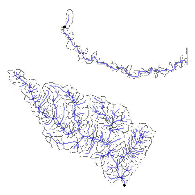
# Below we demonstrate how to extract the upstream and downstream flowpaths for specific points

us_647<-hydro_out$us_flowpaths %>%
  filter(pour_point_id == "647") # get all upstream link_ids from link_id 647
ds_101.1<-hydro_out$ds_flowpaths %>%
  filter(origin_link_id == "101.1") # get all downstream link_ids from
#                                   # link_id 101.1 (this corresponds with site_id = 62)

lines_out<-hydro_out$stream_lines %>%
  filter(link_id %in% us_647$origin_link_id |
           link_id %in% ds_101.1$destination_link_id
  )
sub_out<-hydro_out$subbasins %>%
  filter(link_id %in% us_647$origin_link_id |
           link_id %in% ds_101.1$destination_link_id
  )

tm_shape(sub_out) + tm_polygons(col="white",alpha =0.2,legend.show=F) +
  tm_shape(lines_out) + tm_lines(col="blue",alpha =0.5,legend.show=F,lwd =3) +
  tm_shape(hydro_out$links %>% filter(link_id %in% c("647","101.1"))) +
  tm_dots(legend.show=F,size=0.45,border.col="black",border.alpha=1,border.lwd=1) +
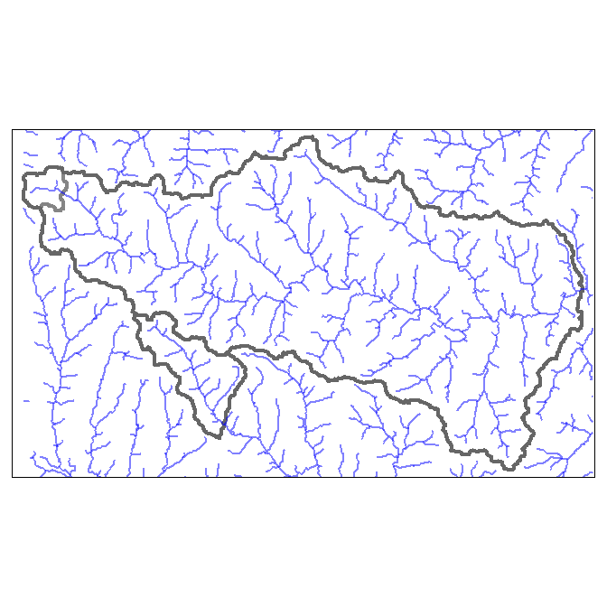
tm_layout(frame = FALSE)Once lookups are established, catchments can easily be retrieved
subbasin_catchments<-get_catchment( # retrieve catchment for an arbitrary reach
  input=hydro_out,
  sample_points=NULL,
  link_id="838"
)

point_catchments<-get_catchment( # retrieve catchments at specified sampling points
  input=hydro_out,
  sample_points=c("1","25"),
  link_id=NULL
)

tm_shape(bind_rows(subbasin_catchments,point_catchments)) +
  tm_polygons(col="white",alpha =0.2,legend.show=F,lwd =4) +
  tm_shape(hydro_out$stream_lines) +
tm_lines(col="blue",alpha =0.5,legend.show=F,lwd =2) The entire workflow above can be accomplished with a single function:
output_filename_hydro_sparse<-file.path(save_dir,"Processed_Hydrology_sparse.gpkg")

# In this case we will use a higher stream initiation threshold to speed up calculation.

hydro_out_sparse<-process_hydrology(
  dem=toy_dem,
  output_filename=output_filename_hydro_sparse,
  # burn_streams=system.file("extdata", "nc", "streams.shp", package = "openSTARS"),
  burn_depth=5,
  depression_corr="breach",
  threshold=500L,
  points=hydro_out$snapped_points,
  site_id_col="site_id",
  snap_distance = 1L,
  break_on_noSnap=F,
  pwise_dist=T,
  pwise_all_links=F,
  return_products=F,
  temp_dir=NULL,
  verbose=F
)

ihydro_layers(hydro_out_sparse)
#> # A tibble: 25 × 3
#>    layer_name       data_type data_group
#>    <chr>            <chr>     <chr>
#>  1 dem_final        Raster    hydro
#>  2 dem_d8           Raster    hydro
#>  3 dem_accum_d8     Raster    hydro
#>  4 dem_accum_d8_sca Raster    hydro
#>  5 dem_streams_d8   Raster    hydro
#>  6 ds_flowpaths     Table     flow_path
#>  7 us_flowpaths     Table     flow_path
#>  8 Subbasins_poly   Table     hydro
#>  9 stream_lines     Table     hydro
#> 10 stream_links     Table     hydro
#> # … with 15 more rows

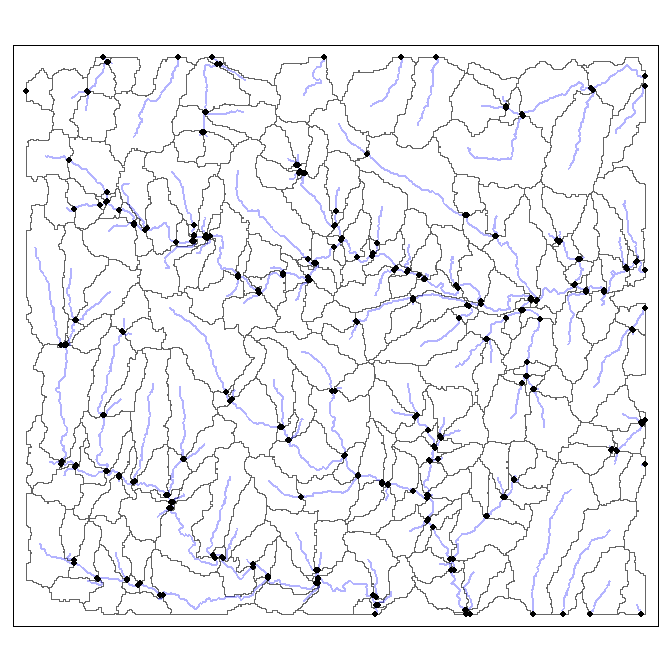
# Since we didn't return the products, we'll verify the outputs exist in the gpkg file

tm_shape(read_sf(hydro_out_sparse$outfile,"Subbasins_poly")) +
  tm_polygons(col="white",alpha =0.2,legend.show=F) +
  tm_shape(read_sf(hydro_out_sparse$outfile,"stream_lines")) +
  tm_lines(col="blue",alpha =0.3,legend.show=F,lwd =2) +
  tm_shape(read_sf(hydro_out_sparse$outfile,"stream_links")) +
tm_dots(legend.show=F,size=0.2,border.col="black",border.alpha=1,border.lwd=1)For more complete and thorough treatment on spatial autocorrelation in stream systems, see Zimmerman and Hoef (2007).
In case we didn’t request pairwise distances in trace_flowpaths(), we
can calculate them separately with generate_pdist(). Below we
calculate a table that summaries relevant pairwise distance measures
between reaches.
# If pairwise distances were not requested with trace_flowpaths(), they can be added
# at any point after using generate_pdist()
hydro_out<-generate_pdist(
input=hydro_out,
pwise_all_links=T # This will calculate pairwise distances between all stream links
# # which can be very slow for dense stream networks
)
# New data available in `fcon_pwise_dist` and 'funcon_pwise_dist'
# *_pwise_dist # -> tables of downstream path lengths between each pair of link_ids,
# # with flow-connected in-stream distances (directed_path_length),
# # flow-unconnected in-stream distances (undirected_path_length),
# # and proportions of shared catchments (prop_shared_catchment)
# # and log-transformed catchment proportions (prop_shared_logcatchment)
con <- DBI::dbConnect(RSQLite::SQLite(), hydro_out$outfile)
ihydro_layers(hydro_out)
#> # A tibble: 28 × 3
#> layer_name data_type data_group
#> <chr> <chr> <chr>
#> 1 dem_final Raster hydro
#> 2 dem_d8 Raster hydro
#> 3 dem_accum_d8 Raster hydro
#> 4 dem_accum_d8_sca Raster hydro
#> 5 dem_streams_d8 Raster hydro
#> 6 ds_flowpaths Table flow_path
#> 7 us_flowpaths Table flow_path
#> 8 Catchment_poly Table hydro
#> 9 Subbasins_poly Table hydro
#> 10 stream_lines Table hydro
#> # … with 18 more rows
# funcon_pwise_dist is only available if pwise_all_links==T
hydro_out$pwise_dist<-bind_rows(collect(tbl(con,"fcon_pwise_dist")) %>% mutate(dist_type="Flow Connected"),
collect(tbl(con,"funcon_pwise_dist")) %>% mutate(dist_type="Flow Unconnected")
)
DBI::dbDisconnect(con)
head(hydro_out$pwise_dist)
#> # A tibble: 6 × 7
#> origin destination directed_path_length prop_shared_…¹ prop_…² undir…³ dist_…⁴
#> <chr> <chr> <dbl> <dbl> <dbl> <dbl> <chr>
#> 1 1 1 132. 1 1 132. Flow C…
#> 2 10 10 42.4 1 1 42.4 Flow C…
#> 3 10 1210 192. 0.0289 0.763 192. Flow C…
#> 4 100 100 230. 1 1 230. Flow C…
#> 5 100 1132 465. 0.284 0.904 465. Flow C…
#> 6 100 1139 579. 0.218 0.886 579. Flow C…
#> # … with abbreviated variable names ¹prop_shared_catchment,
#> # ²prop_shared_logcatchment, ³undirected_path_length, ⁴dist_type
p1<-hydro_out$stream_lines %>%
mutate(link_id=as.character(link_id)) %>%
left_join(hydro_out$pwise_dist %>%
filter(dist_type=="Flow Connected") %>%
filter(origin=="1048") %>%
mutate(directed_path_length=log(directed_path_length)),
by=c("link_id"="destination")) %>%
tm_shape() +
tm_lines(col="directed_path_length",alpha =1,legend.show=T,lwd =2,palette = "viridis",style="cont")+
tm_shape(hydro_out$links %>% filter(link_id=="1048"))+
tm_dots(legend.show=F,size=0.45,border.col="black",border.alpha=1,border.lwd=1)+
tm_layout(main.title = "Flow connected path log-length from 1048",legend.outside = TRUE)
p2<-hydro_out$stream_lines %>%
mutate(link_id=as.character(link_id)) %>%
left_join(hydro_out$pwise_dist %>%
filter(origin=="99") %>%
filter(dist_type=="Flow Unconnected") %>%
mutate(undirected_path_length=log(undirected_path_length)),
by=c("link_id"="destination"),
multiple="all") %>%
tm_shape() +
tm_lines(col="undirected_path_length",alpha =1,legend.show=T,lwd =2,palette = "viridis",style="cont")+
tm_shape(hydro_out$links %>% filter(link_id=="99"))+
tm_dots(legend.show=F,size=0.45,border.col="black",border.alpha=1,border.lwd=1)+
tm_layout(main.title = "Flow Unconnected path log-length from 99",legend.outside = TRUE)
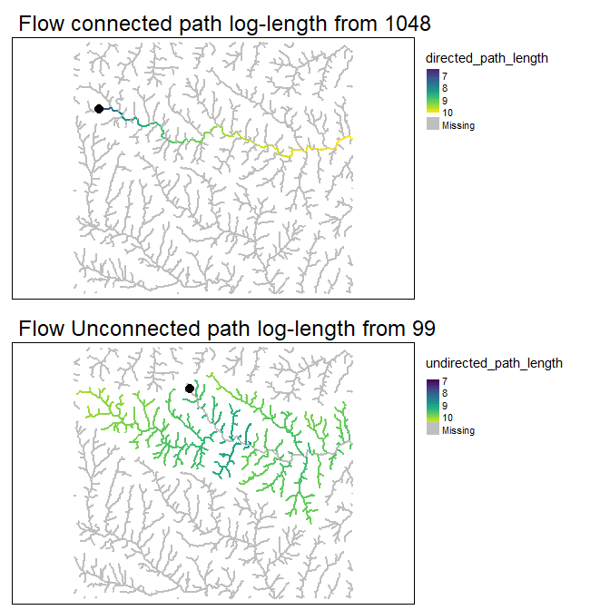
# Verify upstream and downstream distances make sense
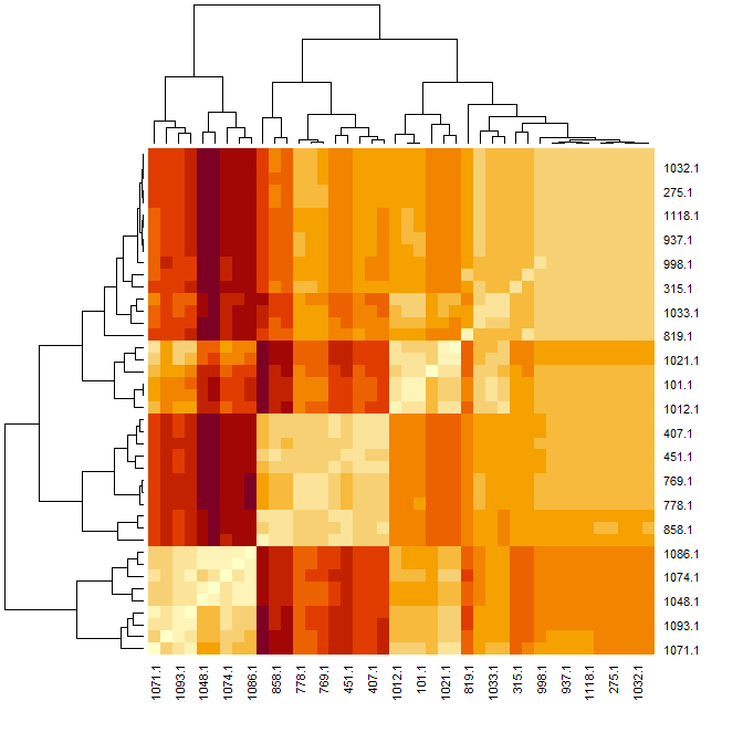
tmap_arrange(p1,p2,ncol=1)Below. we take these distances and visualize them as heatmaps to illustrate how pairwise distance matrices can be used to represent spatial relationships among sites.
# Examine relationships among sampled sites.

# Get link_id for sampled points
sel_link_id<-hydro_out$snapped_points

# filter long table to selected sites, and convert to wide format

# This table describes the flow-connected in-stream distances at destination points (rows)
# from upstream origin points (columns)
dmat<-hydro_out$pwise_dist %>%
  filter(origin %in% sel_link_id$link_id &
           destination %in% sel_link_id$link_id
  ) %>%
  filter(origin!=destination) %>%
  select(-prop_shared_catchment,-undirected_path_length,-prop_shared_logcatchment,-dist_type) %>%
  rename(link_id=origin) %>%
  mutate(directed_path_length=ifelse(directed_path_length==1 | is.na(directed_path_length),0,directed_path_length)) %>%
  distinct() %>%
  filter(directed_path_length!=0) %>%
  pivot_wider(names_from=destination,values_from=directed_path_length,values_fill = 0) %>%
  data.frame(check.names = F) %>%
  tibble::column_to_rownames("link_id") %>%
  log1p()

head(dmat)
#>          1035.1    998.1   1050.1   1012.1 1071.1 968.1 1053.1 1074.1 1037.1
#> 101.1  8.613486 8.995312 9.664710 0.000000      0     0      0      0      0
#> 1012.1 7.494625 8.379798 9.396383 0.000000      0     0      0      0      0
#> 1021.1 8.237140 8.754396 9.548604 7.797961      0     0      0      0      0
#> 1032.1 0.000000 0.000000 8.427519 0.000000      0     0      0      0      0
#> 1033.1 0.000000 8.112417 9.307670 0.000000      0     0      0      0      0
#> 1035.1 0.000000 8.027024 9.282589 0.000000      0     0      0      0      0
#>        1086.1 1093.1 1021.1 924.1 769.1 709.1 780.1 866.1 904.1 850.1
#> 101.1       0      0      0     0     0     0     0     0     0     0
#> 1012.1      0      0      0     0     0     0     0     0     0     0
#> 1021.1      0      0      0     0     0     0     0     0     0     0
#> 1032.1      0      0      0     0     0     0     0     0     0     0
#> 1033.1      0      0      0     0     0     0     0     0     0     0
#> 1035.1      0      0      0     0     0     0     0     0     0     0

# This table describes the proportions of shared catchments at destination points (rows)
# from upstream origin points (columns)
dmat2<-hydro_out$pwise_dist %>%
  filter(origin %in% sel_link_id$link_id &
           destination %in% sel_link_id$link_id
  ) %>%
  filter(origin!=destination) %>%
  select(-directed_path_length,-undirected_path_length,-prop_shared_catchment,-dist_type) %>%
  rename(link_id=origin) %>%
  mutate(prop_shared_logcatchment=ifelse(prop_shared_logcatchment==1 | is.na(prop_shared_logcatchment),
                                         1,prop_shared_logcatchment)) %>%
  distinct() %>%
  filter(prop_shared_logcatchment!=0) %>%
  pivot_wider(names_from=destination,values_from=prop_shared_logcatchment ,values_fill = 0) %>%
  data.frame(check.names = F) %>%
  tibble::column_to_rownames("link_id")

head(dmat2)
#>           1035.1     998.1    1050.1    1012.1 1071.1 968.1 1053.1 1074.1
#> 101.1  0.7653298 0.7563228 0.7294989 0.0000000      0     0      0      0
#> 1012.1 0.9872277 0.9756092 0.9410081 0.0000000      0     0      0      0
#> 1021.1 0.8712224 0.8609692 0.8304339 0.8824939      0     0      0      0
#> 1032.1 0.0000000 0.0000000 0.7370728 0.0000000      0     0      0      0
#> 1033.1 0.0000000 0.8142056 0.7853288 0.0000000      0     0      0      0
#> 1035.1 0.0000000 0.9882312 0.9531825 0.0000000      0     0      0      0
#>        1037.1 1086.1 1093.1 1021.1 924.1 769.1 709.1 780.1 866.1 904.1 850.1
#> 101.1       0      0      0      0     0     0     0     0     0     0     0
#> 1012.1      0      0      0      0     0     0     0     0     0     0     0
#> 1021.1      0      0      0      0     0     0     0     0     0     0     0
#> 1032.1      0      0      0      0     0     0     0     0     0     0     0
#> 1033.1      0      0      0      0     0     0     0     0     0     0     0
#> 1035.1      0      0      0      0     0     0     0     0     0     0     0

# Here we multiply the matrices (using the proportions of shared catchments as a rough weighting scheme)
# calculate manhattan distances and generate a heatmap
(dmat*dmat2) %>%
  dist("man") %>%
  as.matrix() %>%
  heatmap()
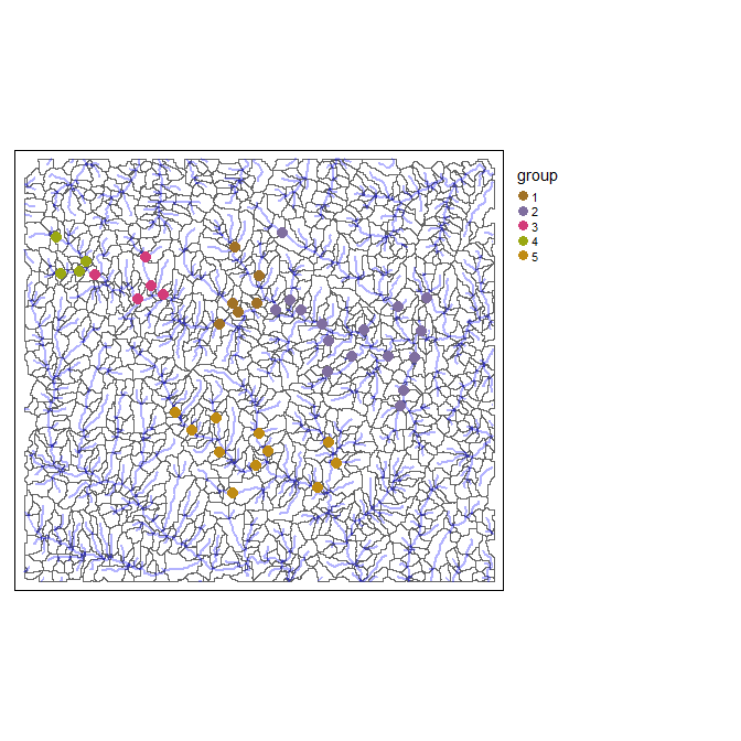
Using these relationships, we can perform a clustering analysis to identify groups of sites with potentially high spatial autocorrelation. These groups could for instance be used for cross-validation purposes.
# Using the above approach, we create 5 groups of spatially proximate points
km<-(dmat*dmat2) %>%
  dist("man") %>%
  hclust() %>%
  cutree(k=5)

gps<-tibble::enframe(km,"link_id","group") %>%
  mutate(link_id=as.numeric(link_id))

point_groups<-hydro_out$snapped_points %>%
  left_join(gps) %>%
  filter(!is.na(group))

# These can be used for cross-validation purposes to see how well the models extrapolate outside of
# sampled areas

tm_shape(hydro_out$subbasins) + tm_polygons(col="white",alpha =0.2,legend.show=F) +
  tm_shape(hydro_out$stream_lines) + tm_lines(col="blue",alpha =0.3,legend.show=F,lwd =2) +
  tm_shape(point_groups) + tm_dots(col="group", palette = "Dark2",legend.show=T,size=0.45)+
  tm_layout(legend.outside = TRUE)
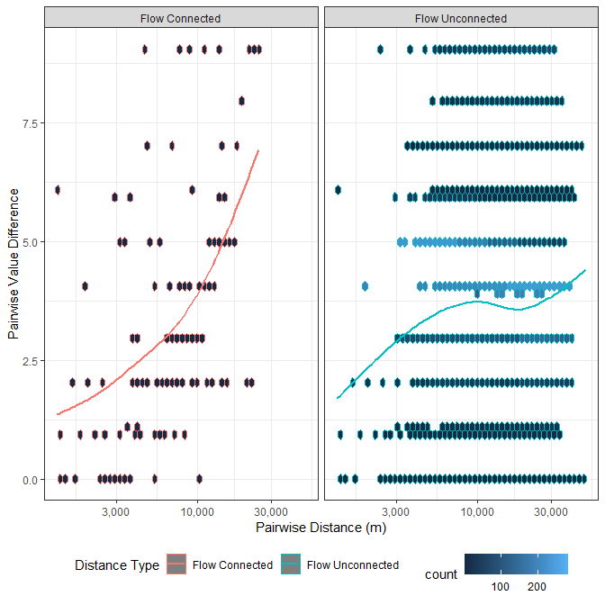
Finally, we’ll examine relationships among our response variable in terms of in-stream distances, contrasting flow connected sites vs, flow unconnected sites. Here we see greater differences between responses with increasing in-stream distance. We expect greater similarity among flow-connected than flow-unconnected sites, but don’t see it here. This may be a product of this being an artificial data set.
# get response variables
response_table<-file.path(save_dir, "sites.shp") %>%
read_sf() %>%
as_tibble() %>%
select(site_id,value) %>%
left_join(hydro_out$snapped_points %>% # join by snapped sites to get link_id values
as_tibble() %>%
select(site_id,link_id)) %>%
mutate(link_id=as.character(link_id))
# Combine pairwise data with values and examine spatial relationships.
dmat<-hydro_out$pwise_dist %>%
filter(origin %in% sel_link_id$link_id &
destination %in% sel_link_id$link_id
) %>%
# Add response values for origin and destination points into the table
left_join(response_table %>% rename(origin_value=value),by=c("origin"="link_id")) %>%
left_join(response_table %>% rename(destination_value=value),by=c("destination"="link_id")) %>%
mutate(value_diff=sqrt((origin_value-destination_value)^2)) %>% # Calculate the squared difference
filter(origin!=destination) %>%
select(-dist_type,-site_id.x,-site_id.y,-origin_value,-destination_value) %>%
pivot_longer(c(directed_path_length,undirected_path_length,prop_shared_catchment,prop_shared_logcatchment),
names_to ="dist_type",
values_to ="dist") %>%
filter(!is.na(dist)) %>%
mutate(`Distance Type`=case_when(
dist_type=="directed_path_length" ~ "Flow Connected",
dist_type=="undirected_path_length" ~ "Flow Unconnected",
dist_type=="prop_shared_catchment" ~ "Shared Catchment",
dist_type=="prop_shared_logcatchment" ~ "Shared log-Catchment",
)) %>%
distinct()
dmat
#> # A tibble: 21,272 × 6
#> origin destination value_diff dist_type dist Distance …¹
#> <chr> <chr> <dbl> <chr> <dbl> <chr>
#> 1 101.1 1035.1 2 directed_path_length 5504. Flow Conne…
#> 2 101.1 1035.1 2 undirected_path_length 5504. Flow Uncon…
#> 3 101.1 1035.1 2 prop_shared_catchment 0.0179 Shared Cat…
#> 4 101.1 1035.1 2 prop_shared_logcatchment 0.765 Shared log…
#> 5 101.1 998.1 2 directed_path_length 8064. Flow Conne…
#> 6 101.1 998.1 2 undirected_path_length 8064. Flow Uncon…
#> 7 101.1 998.1 2 prop_shared_catchment 0.0146 Shared Cat…
#> 8 101.1 998.1 2 prop_shared_logcatchment 0.756 Shared log…
#> 9 101.1 1050.1 2 directed_path_length 15751. Flow Conne…
#> 10 101.1 1050.1 2 undirected_path_length 15751. Flow Uncon…
#> # … with 21,262 more rows, and abbreviated variable name ¹`Distance Type`
require(ggplot2)
ggplot(dmat %>% filter(dist_type %in% c("directed_path_length","undirected_path_length")),
aes(x=dist,y=value_diff,col=`Distance Type`))+
geom_hex(bins=50)+
geom_smooth(method="gam",se=F)+
theme_bw()+
theme(legend.position = "bottom")+
ylab("Pairwise Value Difference")+
xlab("Pairwise Distance (m)")+
scale_x_log10(labels=scales::comma)+
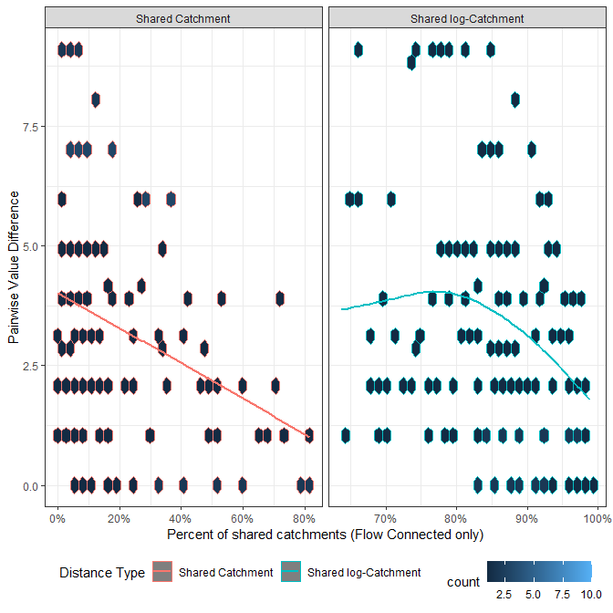
facet_wrap(~`Distance Type`)Finally, we’ll do a similar comparison but using percent of shared catchments. Here we expect pairwise differences to decrease as the percent of shared catchments increases.
ggplot(dmat %>%
         filter(dist_type %in% c("prop_shared_catchment","prop_shared_logcatchment")) %>%
         filter(dist>0),
       aes(x=dist,y=value_diff,colour=`Distance Type`))+
  geom_hex()+
  geom_smooth(method="gam",se=F)+
  theme_bw()+
  theme(legend.position = "bottom")+
  ylab("Pairwise Value Difference")+
  xlab("Percent of shared catchments (Flow Connected only)")+
  scale_x_continuous(labels=scales::percent)+
facet_wrap(~`Distance Type`,scales ="free_x")Layers of interest (loi) represent the features on the landscape we are interested in relating to the observed responses in the stream. These can include: land-cover, climate, geology, soils, NDVI, slope, etc.
## Predictors from openSTARS
system.file("extdata", "nc", "landuse_r.tif", package = "openSTARS") %>%
  rast() %>%
  setNames("LC") %>%
  writeRaster(file.path(save_dir, "LC.tif"),overwrite=T)

landuse_r_path <-file.path(save_dir, "LC.tif")
geology_path<-system.file("extdata", "nc", "geology.shp", package = "openSTARS")
pointsources_path<-system.file("extdata", "nc", "pointsources.shp", package = "openSTARS")

read_sf(pointsources_path) %>%
  mutate(pointsource="pontsrc") %>%
  st_buffer(60) %>%
  write_sf(file.path(save_dir, "pointsources.shp"),overwrite=T)

pointsources_path<-file.path(save_dir, "pointsources.shp")


# Numeric Raster

wbt_slope(
  dem = file.path(save_dir, "toy_dem.tif"),
  output = file.path(save_dir, "slope.tif")
)

# Combine loi layers
output_filename_loi<-file.path(save_dir,"Processed_loi.gpkg")

# This function standardizes numeric and categorical loi layers.

loi_combined<-process_loi(
  dem=toy_dem,
  num_inputs=list(# Can be given as a mixture of input types (file paths, or any sf or terra format)
    slope=file.path(save_dir, "slope.tif")
  ),
  cat_inputs=list(# Can be given as a mixture of input types (file paths, or any sf or terra format)
    landcover=landuse_r_path,
    geology=geology_path,
    pointsources=pointsources_path
  ),
  variable_names=list( # any unlisted inputs will be used in their entirety
    geology="GEO_NAME", # names listed here will subset those attributes or layers from the inputs
    pointsources="pontsrc"
  ),
  output_filename=output_filename_loi,
  return_products=T,
  temp_dir=NULL,
  verbose=T
)

ihydro_layers(loi_combined)
#> # A tibble: 20 × 3
#>    layer_name      data_type data_group
#>    <chr>           <chr>     <chr>
#>  1 GEO_NAME_CZam   Raster    loi
#>  2 GEO_NAME_CZbg   Raster    loi
#>  3 GEO_NAME_CZfg   Raster    loi
#>  4 GEO_NAME_CZg    Raster    loi
#>  5 GEO_NAME_CZig   Raster    loi
#>  6 GEO_NAME_CZlg   Raster    loi
#>  7 GEO_NAME_CZve   Raster    loi
#>  8 GEO_NAME_Km     Raster    loi
#>  9 LC_1            Raster    loi
#> 10 LC_2            Raster    loi
#> 11 LC_3            Raster    loi
#> 12 LC_4            Raster    loi
#> 13 LC_5            Raster    loi
#> 14 LC_6            Raster    loi
#> 15 LC_7            Raster    loi
#> 16 pontsrc_pontsrc Raster    loi
#> 17 slope           Raster    loi
#> 18 DEM_Extent      Table     meta
#> 19 loi_meta        Table     meta
#> 20 DEM_Extent      Vector    meta
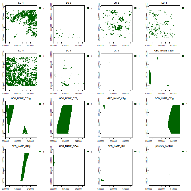
All categorical layers have been transformed to rasters with 1 indicating presence, and NA for absence. The layers have been rescaled and projected to match the DEM
plot(loi_combined$cat_inputs,type="classes",col="darkgreen")All numeric layers have been rescaled and projected to match the DEM.
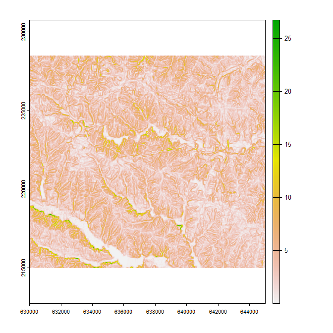
plot(loi_combined$num_inputs,type="continuous")Instead of processing the loi separately (as was done above), they can instead be added to the completed workflow, and added to the existing gpkg file for convenient file storage/organization.
# In this case, we will use our previously calculated loi results, but if `process_loi`
# is run with an input parameter specified, the loi rasters will be added to the
# output. This can make for convenient data storage.

hydro_out_sparse<-process_loi(
  input=hydro_out_sparse,
  num_inputs=list(# Can be given as a mixture of input types (file paths, or any sf or terra format)
    slope=file.path(save_dir, "slope.tif")
  ),
  cat_inputs=list(# Can be given as a mixture of input types (file paths, or any sf or terra format)
    landcover=landuse_r_path,
    geology=geology_path,
    pointsources=pointsources_path
  ),
  variable_names=list( # any unlisted inputs will be used in their entirety
    geology="GEO_NAME", # names listed here will subset those attributes or layers from the inputs
    pointsources="pontsrc"
  ),
  return_products=F, # these layers can get large, and it is generally not advised to return them into R
  temp_dir=NULL,
  verbose=F
)

print(ihydro_layers(hydro_out_sparse),n=40)
#> # A tibble: 43 × 3
#>    layer_name         data_type data_group
#>    <chr>              <chr>     <chr>
#>  1 dem_final          Raster    hydro
#>  2 dem_d8             Raster    hydro
#>  3 dem_accum_d8       Raster    hydro
#>  4 dem_accum_d8_sca   Raster    hydro
#>  5 dem_streams_d8     Raster    hydro
#>  6 GEO_NAME_CZam      Raster    loi
#>  7 GEO_NAME_CZbg      Raster    loi
#>  8 GEO_NAME_CZfg      Raster    loi
#>  9 GEO_NAME_CZg       Raster    loi
#> 10 GEO_NAME_CZig      Raster    loi
#> 11 GEO_NAME_CZlg      Raster    loi
#> 12 GEO_NAME_CZve      Raster    loi
#> 13 GEO_NAME_Km        Raster    loi
#> 14 LC_1               Raster    loi
#> 15 LC_2               Raster    loi
#> 16 LC_3               Raster    loi
#> 17 LC_4               Raster    loi
#> 18 LC_5               Raster    loi
#> 19 LC_6               Raster    loi
#> 20 LC_7               Raster    loi
#> 21 pontsrc_pontsrc    Raster    loi
#> 22 slope              Raster    loi
#> 23 ds_flowpaths       Table     flow_path
#> 24 us_flowpaths       Table     flow_path
#> 25 Subbasins_poly     Table     hydro
#> 26 stream_lines       Table     hydro
#> 27 stream_links       Table     hydro
#> 28 stream_links_attr  Table     hydro
#> 29 stream_points      Table     hydro
#> 30 stream_points_attr Table     hydro
#> 31 DEM_Extent         Table     meta
#> 32 loi_meta           Table     meta
#> 33 site_id_col        Table     meta
#> 34 fcon_pwise_dist    Table     pwise_dist
#> 35 original_points    Table     sample_points
#> 36 snapped_points     Table     sample_points
#> 37 Subbasins_poly     Vector    hydro
#> 38 stream_lines       Vector    hydro
#> 39 stream_links       Vector    hydro
#> 40 stream_points      Vector    hydro
#> # … with 3 more rowsNew research is showing that the presence of particular features on the landscape is not always sufficient to predict the in-stream response to those features, and the location of those features relative to the locations of streams and areas of higher flow accumulation is very important (Peterson et al. 2011).
ihydro provides two functions for calculating weighted spatial
summaries: attrib_points() and fasttrib_points(). attrib_points()
uses the hydroweight package
to calculate weighted spatial summaries of supplied loi layers. It can
be used to examine the resulting distance-weighted rasters and
distance-weighted loi layers. However, attrib_points() is slow, so
fasttrib_points() is available for improved performance for larger
datasets.
The attrib_points() function uses the
hydroweight package and can
calculate and return weighted attributes for any points identified
either through supplied sampling points and/or arbitrary link_ids. The
returned products can be helpful in visualizing how the final weighted
attributes are derived.
attrib_points_time_small<-system.time(
  final_attributes_sub_slow<-attrib_points(
    input=hydro_out,
    out_filename=file.path(tempdir(),"attrib_points1.csv"),
    loi_file=output_filename_loi,
    loi_cols=NULL,
    sample_points=c("1","25","80"),
    link_id=NULL,
    clip_region=NULL,
    target_o_type=c("point"),
    weighting_scheme = c("lumped","iFLO", "iFLS", "HAiFLO", "HAiFLS"),
    loi_numeric_stats = c("distwtd_mean", "distwtd_sd", "mean", "sd", "median", "min", "max", "sum"),
    inv_function = function(x) {
      (x * 0.001 + 1)^-1
    },
    temp_dir=NULL,
    return_products=T,
    verbose=T
  )
)


final_attributes_sub_slow
#> # A tibble: 3 × 97
#>   link_id site_id products     slope_l…¹ slope…² slope…³ slope…⁴ slope…⁵ slope…⁶
#>   <chr>   <chr>   <list>           <dbl>   <dbl>   <dbl>   <dbl>   <dbl>   <dbl>
#> 1 1107.1  1       <named list>      2.96   1.49     2.83 0.203     10.2    3613.
#> 2 1050.1  25      <named list>      3.48   2.23     3.10 0.00216   22.8  257020.
#> 3 555.1   80      <named list>      2.23   0.837    2.16 0.400      4.34    353.
#> # … with 88 more variables: slope_iFLO_distwtd_mean <dbl>,
#> #   slope_iFLO_distwtd_sd <dbl>, slope_iFLS_distwtd_mean <dbl>,
#> #   slope_iFLS_distwtd_sd <dbl>, slope_HAiFLO_distwtd_mean <dbl>,
#> #   slope_HAiFLO_distwtd_sd <dbl>, slope_HAiFLS_distwtd_mean <dbl>,
#> #   slope_HAiFLS_distwtd_sd <dbl>, LC_1_lumped_prop <dbl>,
#> #   LC_2_lumped_prop <dbl>, LC_3_lumped_prop <dbl>, LC_4_lumped_prop <dbl>,
#> #   LC_5_lumped_prop <dbl>, LC_6_lumped_prop <dbl>, LC_7_lumped_prop <dbl>, …
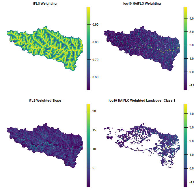
We can access the weighting layers and weighted attribute layers (if
return_products==T) of the attrib_points() output.
plot(
  rast(
    list(
      rast(final_attributes_sub_slow$products[[2]]$iFLS)%>%
        setNames("iFLS Weighting"),
      log10(rast(final_attributes_sub_slow$products[[2]]$HAiFLO))%>%
        setNames("log10-HAiFLO Weighting"),
      rast(final_attributes_sub_slow$products[[2]]$iFLS_num) %>%
        setNames("iFLS Weighted Slope"),
      log10(rast(final_attributes_sub_slow$products[[2]]$HAiFLO_cat)[[1]]) %>%
        setNames("log10-HAiFLO Weighted Landcover Class 1")
    )
  ),
  col=viridis::viridis(101),
  axes=F
)
The fasttrib_points() function is faster for larger data sets, more
loi, and more sampling points. For very small datasets attrib_points()
may be faster.
fasttrib_points_time_small<-system.time(
  final_attributes_sub<-fasttrib_points(
    input=hydro_out,
    out_filename="sample_points_wgtattr.csv",
    loi_file=output_filename_loi, # specify loi file, if NULL, function will look for loi in 'input'
    loi_cols=NULL,                # Specify loi columns to use, if NULL, all will be used
    iDW_file=NULL, # Leaving this as NULL will look for iDW in 'input' and calculate any not available
    store_iDW=T,   # This will save the distance weights to the input or iDW_file if it is specified
    sample_points=c("1","25","80"),
    link_id=NULL,
    target_o_type=c("point"),
    weighting_scheme =  c("lumped",  "iFLS", "HAiFLS","iFLO",  "HAiFLO"),
    loi_numeric_stats = c("mean", "sd", "median", "min", "max", "sum"),
    inv_function = function(x) {
      (x * 0.001 + 1)^-1
    },
    temp_dir=NULL,
    verbose=T
  )
)

ihydro_layers(hydro_out)
#> # A tibble: 35 × 3
#>    layer_name                   data_type data_group
#>    <chr>                        <chr>     <chr>
#>  1 dem_final                    Raster    hydro
#>  2 dem_d8                       Raster    hydro
#>  3 dem_accum_d8                 Raster    hydro
#>  4 dem_accum_d8_sca             Raster    hydro
#>  5 dem_streams_d8               Raster    hydro
#>  6 iFLS                         Raster    iDW
#>  7 HAiFLS                       Raster    iDW
#>  8 HAiFLO_unn_group0Lec41Mc3Psz Raster    iDW
#>  9 HAiFLO_unn_group1iBKALOf0eCL Raster    iDW
#> 10 iFLO_unn_group0Lec41Mc3Psz   Raster    iDW
#> # … with 25 more rows

final_attributes_sub
#> # A tibble: 3 × 97
#>   link_id site_id status slope…¹ slope…² slope…³ slope…⁴ slope…⁵ slope…⁶ slope…⁷
#>   <chr>   <chr>   <chr>    <dbl>   <dbl>   <dbl>   <dbl>   <dbl>   <dbl>   <dbl>
#> 1 1107.1  1       Compl…    3.02   1.46  0.203     10.2     2.89   3254.    3.08
#> 2 1050.1  25      Compl…    3.51   2.24  0.00216   22.8     3.14 253079.    3.56
#> 3 555.1   80      Compl…    2.34   0.904 0.400      4.34    2.19    273.    2.37
#> # … with 87 more variables: slope_HAiFLS_mean <dbl>, slope_iFLO_mean <dbl>,
#> #   slope_HAiFLO_mean <dbl>, slope_HAiFLO_sd <dbl>, slope_HAiFLS_sd <dbl>,
#> #   slope_iFLO_sd <dbl>, slope_iFLS_sd <dbl>, LC_1_lumped_prop <dbl>,
#> #   LC_1_iFLS_prop <dbl>, LC_1_HAiFLS_prop <dbl>, LC_1_iFLO_prop <dbl>,
#> #   LC_1_HAiFLO_prop <dbl>, LC_2_lumped_prop <dbl>, LC_2_iFLS_prop <dbl>,
#> #   LC_2_HAiFLS_prop <dbl>, LC_2_iFLO_prop <dbl>, LC_2_HAiFLO_prop <dbl>,
#> # LC_3_lumped_prop <dbl>, LC_3_iFLS_prop <dbl>, LC_3_HAiFLS_prop <dbl>, …final_attributes<-fasttrib_points(
input=hydro_out,
out_filename="sample_points_wgtattr.csv",
loi_file=output_filename_loi,
loi_cols=NULL,
iDW_file=NULL,
store_iDW=T,
sample_points=hydro_out$snapped_points$site_id, # here we specify all sampling points
link_id=NULL,
target_o_type=c("point"),
weighting_scheme = c("lumped", "iFLS", "iFLO", "HAiFLO", "HAiFLS"),
loi_numeric_stats = c("mean", "sd", "min", "max"),
inv_function = function(x) {
(x * 0.001 + 1)^-1
},
temp_dir=NULL,
verbose=F
)
final_attributes
#> # A tibble: 45 × 95
#> link_id site_id status slope_lump…¹ slope…² slope…³ slope…⁴ slope…⁵ slope…⁶
#> <chr> <chr> <chr> <dbl> <dbl> <dbl> <dbl> <dbl> <dbl>
#> 1 1118.1 41 Complete 2.43 1.57 0.00253 11.4 2.46 2.31
#> 2 1107.1 1 Complete 3.02 1.46 0.203 10.2 3.08 2.79
#> 3 101.1 62 Complete 3.13 1.81 0.0667 8.27 3.19 3.05
#> 4 142.1 26 Complete 2.82 1.37 0.152 7.64 2.86 2.53
#> 5 1086.1 4 Complete 3.37 1.75 0.146 12.3 3.42 3.10
#> 6 1053.1 7 Complete 2.75 1.75 0.0323 9.97 2.84 2.79
#> 7 1048.1 5 Complete 2.52 1.59 0.0323 7.90 2.57 2.53
#> 8 1074.1 8 Complete 3.23 1.90 0.0323 12.3 3.29 3.05
#> 9 1080.1 66 Complete 3.97 2.04 0.110 10.7 4.06 3.53
#> 10 1093.1 28 Complete 3.33 1.80 0.152 10.8 3.38 3.14
#> # … with 35 more rows, 86 more variables: slope_iFLO_mean <dbl>,
#> # slope_HAiFLO_mean <dbl>, slope_HAiFLO_sd <dbl>, slope_HAiFLS_sd <dbl>,
#> # slope_iFLO_sd <dbl>, slope_iFLS_sd <dbl>, LC_1_lumped_prop <dbl>,
#> # LC_1_iFLS_prop <dbl>, LC_1_HAiFLS_prop <dbl>, LC_1_iFLO_prop <dbl>,
#> # LC_1_HAiFLO_prop <dbl>, LC_2_lumped_prop <dbl>, LC_2_iFLS_prop <dbl>,
#> # LC_2_HAiFLS_prop <dbl>, LC_2_iFLO_prop <dbl>, LC_2_HAiFLO_prop <dbl>,
#> # LC_3_lumped_prop <dbl>, LC_3_iFLS_prop <dbl>, LC_3_HAiFLS_prop <dbl>, …In order to make predictions across the landscape, we will need to
calculate our attributes across the landscape as well. We leave
sample_points and link_id as NULL to predict across all reaches. At
this point, we may also consider switching our target_o parameter from
the sampling point (as was done above) to the entire reach by setting
target_o_type=“segment_whole”. This will calculate all target_o
weighting schemes to be the entire reach. This may be more conservative
for predicting beyond sampling points as it integrates landscape factors
across the length of the whole reach.
# This function is optional. It will save the hydroweight rasters in either a separate gpkp,
# or the input pkg.

# These can be large and take up a lot of room, so consider whether they are needed before storing.
# Having the raster available does decrease the computation time of fasttrib_points().

dw_time<-system.time(
  Processed_HW<-prep_weights(
    input=hydro_out,
    output_filename=file.path(tempfile(),"Processed_HW_out.gpkg")
  )
)


fasttrib_points_time_big<-system.time(
  final_attributes_all<-fasttrib_points(
    input=hydro_out,
    out_filename="sample_points_wgtattr.csv",
    loi_file=output_filename_loi,
    loi_cols=NULL,
    iDW_file=file.path(tempfile(),"iDW_temp.gpkg"),
    #iDW_file = file.path(tempfile(),"Processed_HW_out.gpkg"), # to use previously calculated weights
    store_iDW=T,
    sample_points=NULL, # by specifying neither sample_points nor link_id
    link_id=NULL,       #   we get all reaches
    target_o_type=c("segment_point"),
    weighting_scheme =  c("lumped", "iFLS", "iFLO",  "HAiFLO",  "HAiFLS"),
    loi_numeric_stats = c("mean", "sd", "min", "max"),
    inv_function = function(x) {
      (x * 0.001 + 1)^-1
    },
    temp_dir=NULL,
    verbose=F
  )
)

final_attributes_all
#> # A tibble: 1,241 × 95
#>    link_id site_id status   slope_lump…¹ slope…² slope…³ slope…⁴ slope…⁵ slope…⁶
#>    <chr>   <chr>   <chr>           <dbl>   <dbl>   <dbl>   <dbl>   <dbl>   <dbl>
#>  1 6       <NA>    Complete         3.93    1.90  0.178     8.26    3.97    3.25
#>  2 5       <NA>    Complete         4.73    2.43  0.385    10.4     4.85    4.56
#>  3 1202    <NA>    Complete         3.97    1.91  0.0656   12.7     4.03    3.89
#>  4 1210    <NA>    Complete         4.09    2.34  0.119    15.9     4.15    3.92
#>  5 1208    <NA>    Complete         3.58    2.21  0.0485   14.5     3.65    3.46
#>  6 1       <NA>    Complete         4.40    2.32  0.330     9.19    4.44    4.04
#>  7 1199    <NA>    Complete         3.65    2.18  0.117    12.9     3.75    3.62
#>  8 2       <NA>    Complete         3.46    1.73  0.296     8.18    3.55    3.57
#>  9 1200    <NA>    Complete         4.33    2.59  0.162    17.8     4.45    3.92
#> 10 33      <NA>    Complete         4.64    2.82  0.204    15.0     4.79    4.48
#> # … with 1,231 more rows, 86 more variables: slope_iFLO_mean <dbl>,
#> #   slope_HAiFLO_mean <dbl>, slope_HAiFLO_sd <dbl>, slope_HAiFLS_sd <dbl>,
#> #   slope_iFLO_sd <dbl>, slope_iFLS_sd <dbl>, LC_1_lumped_prop <dbl>,
#> #   LC_1_iFLS_prop <dbl>, LC_1_HAiFLS_prop <dbl>, LC_1_iFLO_prop <dbl>,
#> #   LC_1_HAiFLO_prop <dbl>, LC_2_lumped_prop <dbl>, LC_2_iFLS_prop <dbl>,
#> #   LC_2_HAiFLS_prop <dbl>, LC_2_iFLO_prop <dbl>, LC_2_HAiFLO_prop <dbl>,
#> #   LC_3_lumped_prop <dbl>, LC_3_iFLS_prop <dbl>, LC_3_HAiFLS_prop <dbl>, …

attrib_points_time_big<-system.time(
  final_attributes_slow<-attrib_points(
    input=hydro_out,
    out_filename=file.path(tempdir(),"attrib_points1.csv"),
    loi_file=output_filename_loi,
    loi_cols=NULL,
    sample_points=NULL,
    link_id=NULL,
    clip_region=NULL,
    target_o_type=c("segment_point"),
    weighting_scheme = c("lumped","iFLO", "iFLS", "HAiFLO", "HAiFLS"),
    loi_numeric_stats = c("distwtd_mean", "distwtd_sd", "mean", "sd", "min", "max"),
    inv_function = function(x) {
      (x * 0.001 + 1)^-1
    },
    temp_dir=NULL,
    return_products=T,
    verbose=F
  )
)

final_attributes_slow
#> # A tibble: 1,241 × 95
#>    link_id site_id products     slope_…¹ slope…² slope…³ slope…⁴ slope…⁵ slope…⁶
#>    <chr>   <chr>   <list>          <dbl>   <dbl>   <dbl>   <dbl>   <dbl>   <dbl>
#>  1 6       <NA>    <named list>     3.73    1.91  0.100     8.26    3.89    1.92
#>  2 5       <NA>    <named list>     4.20    2.40  0.356    10.4     4.60    2.51
#>  3 1202    <NA>    <named list>     3.86    1.92  0.0656   12.7     4.01    1.91
#>  4 1210    <NA>    <named list>     3.99    2.34  0.119    16.6     4.33    2.40
#>  5 1208    <NA>    <named list>     3.46    2.21  0.0485   14.5     3.76    2.37
#>  6 1       <NA>    <named list>     4.28    2.39  0.330    10.2     4.32    2.35
#>  7 1199    <NA>    <named list>     3.44    2.15  0.117    12.9     3.79    2.26
#>  8 2       <NA>    <named list>     3.18    1.75  0.0870    8.18    3.40    1.78
#>  9 1200    <NA>    <named list>     4.20    2.60  0.162    17.8     4.60    2.75
#> 10 33      <NA>    <named list>     4.44    2.77  0.0765   15.0     4.71    2.86
#> # … with 1,231 more rows, 86 more variables: slope_iFLS_distwtd_mean <dbl>,
#> #   slope_iFLS_distwtd_sd <dbl>, slope_HAiFLO_distwtd_mean <dbl>,
#> #   slope_HAiFLO_distwtd_sd <dbl>, slope_HAiFLS_distwtd_mean <dbl>,
#> #   slope_HAiFLS_distwtd_sd <dbl>, LC_1_lumped_prop <dbl>,
#> #   LC_2_lumped_prop <dbl>, LC_3_lumped_prop <dbl>, LC_4_lumped_prop <dbl>,
#> #   LC_5_lumped_prop <dbl>, LC_6_lumped_prop <dbl>, LC_7_lumped_prop <dbl>,
#> #   GEO_NAME_CZam_lumped_prop <dbl>, GEO_NAME_CZbg_lumped_prop <dbl>, …

pmap(
  list(
    list("attrib_points()","fasttrib_points()",
         "attrib_points()","fasttrib_points()"),
    list(attrib_points_time_small,
         fasttrib_points_time_small,
         attrib_points_time_big,
         fasttrib_points_time_big),
    list(final_attributes_sub_slow %>%
           select(-any_of("products"),-any_of("link_id"),-any_of("site_id"),-any_of("status")),
         final_attributes_sub%>%
           select(-any_of("products"),-any_of("link_id"),-any_of("site_id"),-any_of("status")),
         final_attributes_slow %>%
           select(-any_of("products"),-any_of("link_id"),-any_of("site_id"),-any_of("status")),
         final_attributes_all%>%
           select(-any_of("products"),-any_of("link_id"),-any_of("site_id"),-any_of("status"))
    )),
  function(.z,.x,.y) paste0(.z," took ",
                            round(.x[[3]]/60,2),
                            " min to calculate for ",
                            nrow(.y)," reaches with ",
                            ncol(.y),
                            " attributes using ", nbrOfWorkers(),
                            " cores.")
)
#> [[1]]
#> [1] "attrib_points() took 1 min to calculate for 3 reaches with 94 attributes using 4 cores."
#>
#> [[2]]
#> [1] "fasttrib_points() took 1.8 min to calculate for 3 reaches with 94 attributes using 4 cores."
#>
#> [[3]]
#> [1] "attrib_points() took 26.85 min to calculate for 1241 reaches with 92 attributes using 4 cores."
#>
#> [[4]]
#> [1] "fasttrib_points() took 12.63 min to calculate for 1241 reaches with 92 attributes using 4 cores."

paste0(round(dw_time[[3]]/60,2),
       " min to calculate distance weights for ",
       nrow(final_attributes_all)," reaches using ",
       nbrOfWorkers(),
       " cores.")
#> [1] "2.66 min to calculate distance weights for 1241 reaches using 4 cores."We’ll finish off with a brief demonstration of how to use the geospatial products calculated above to build, and validate a predictive model. First we’ll create a combined dataset:
# As we will ultimately be predicting to our sparse landscape, we will only keep
# autocorrelation variables that are relevant to the sparse landscape. This would
# not necessarily be required if predicting to the more dense landscape.


# get response variables
response_table<-file.path(save_dir, "sites.shp") %>%
  read_sf() %>%
  as_tibble() %>%
  select(site_id,value) %>%
  left_join(hydro_out$links %>%
              as_tibble() %>%
              select(site_id,link_id) %>%
              mutate(site_id=as.character(site_id))) %>%
  mutate(link_id=as.character(link_id)) %>%
  filter(!is.na(link_id))

head(response_table)
#> # A tibble: 6 × 3
#>   site_id value link_id
#>   <chr>   <dbl> <chr>
#> 1 1           1 1107.1
#> 2 4           1 1086.1
#> 3 5           1 1048.1
#> 4 7           1 1053.1
#> 5 8           1 1074.1
#> 6 11          2 1037.1

# Columns for spatial cross-validation
# Here we will use a matrix of directed path lengths to perform the
# spatial cross-validation:
clust_data<-hydro_out$pwise_dist %>%
  filter(origin %in% response_table$link_id) %>%
  filter(origin!=destination) %>%
  select(-prop_shared_catchment,-undirected_path_length,-prop_shared_logcatchment,-dist_type) %>%
  rename(link_id=origin) %>%
  mutate(directed_path_length=ifelse(directed_path_length==1 | is.na(directed_path_length),0,directed_path_length)) %>%
  distinct() %>%
  filter(directed_path_length!=0) %>%
  pivot_wider(names_from=destination,values_from=directed_path_length ,values_fill = 0) %>%
  data.frame(check.names = F) %>%
  tibble::column_to_rownames("link_id")  %>%
  log1p() %>%
  tibble::rownames_to_column("link_id") %>%
  as_tibble() %>%
  rename_with(.cols=c(everything(),-link_id),.fn=~paste0("CLUST_",.))

head(clust_data)
#> # A tibble: 6 × 198
#>   link_id CLUST_101 CLUST_1131 CLUST_1…¹ CLUST…² CLUST…³ CLUST…⁴ CLUST…⁵ CLUST…⁶
#>   <chr>       <dbl>      <dbl>     <dbl>   <dbl>   <dbl>   <dbl>   <dbl>   <dbl>
#> 1 101.1        7.74       7.77      7.99    8.03    8.12    8.17    8.33    8.35
#> 2 1012.1       0          0         0       0       0       0       0       0
#> 3 1021.1       0          0         0       0       0       0       0       0
#> 4 1032.1       0          0         0       0       0       0       0       0
#> 5 1033.1       0          0         0       0       0       0       0       0
#> 6 1035.1       0          0         0       0       0       0       0       0
#> # … with 189 more variables: CLUST_1063 <dbl>, CLUST_1124 <dbl>,
#> #   CLUST_1035.1 <dbl>, CLUST_1035 <dbl>, CLUST_987 <dbl>, CLUST_1079 <dbl>,
#> #   CLUST_1011 <dbl>, CLUST_966 <dbl>, CLUST_1034 <dbl>, CLUST_974 <dbl>,
#> #   CLUST_998.1 <dbl>, CLUST_998 <dbl>, CLUST_1015 <dbl>, CLUST_962 <dbl>,
#> #   CLUST_943 <dbl>, CLUST_1025 <dbl>, CLUST_977 <dbl>, CLUST_1002 <dbl>,
#> #   CLUST_939 <dbl>, CLUST_965 <dbl>, CLUST_945 <dbl>, CLUST_971 <dbl>,
#> #   CLUST_1143 <dbl>, CLUST_948 <dbl>, CLUST_972 <dbl>, CLUST_989 <dbl>, …

# Combine the data into a single dataset.
comb_data<-response_table %>%
  left_join(
    final_attributes %>% mutate(site_id=as.character(site_id))   # replaces missing proportions with 0's
  ) %>%
  left_join(
    hydro_out$pwise_dist %>%
      filter(origin %in% response_table$link_id) %>%
      select(origin,destination,prop_shared_catchment) %>%
      filter(origin!=destination) %>%
      rename(link_id=destination) %>%
      mutate(origin=paste0("Prop_catch_",origin))%>%
      mutate(prop_shared_catchment=ifelse(prop_shared_catchment==1 | is.na(prop_shared_catchment),0,prop_shared_catchment)) %>%
      distinct() %>%
      filter(prop_shared_catchment!=0) %>%
      pivot_wider(names_from=origin,values_from=prop_shared_catchment,values_fill=0)
  ) %>%
  left_join(clust_data) %>%
  filter(!is.na(link_id)) %>%
  mutate(across(starts_with("Prop_catch_"),~ifelse(is.na(.),0,.)))

head(comb_data)
#> # A tibble: 6 × 338
#>   site_id value link_id status   slope…¹ slope…² slope…³ slope…⁴ slope…⁵ slope…⁶
#>   <chr>   <dbl> <chr>   <chr>      <dbl>   <dbl>   <dbl>   <dbl>   <dbl>   <dbl>
#> 1 1           1 1107.1  Complete    3.02    1.46  0.203    10.2     3.08    2.79
#> 2 4           1 1086.1  Complete    3.37    1.75  0.146    12.3     3.42    3.10
#> 3 5           1 1048.1  Complete    2.52    1.59  0.0323    7.90    2.57    2.53
#> 4 7           1 1053.1  Complete    2.75    1.75  0.0323    9.97    2.84    2.79
#> 5 8           1 1074.1  Complete    3.23    1.90  0.0323   12.3     3.29    3.05
#> 6 11          2 1037.1  Complete    3.42    2.22  0.0323   22.8     3.49    3.17
#> # … with 328 more variables: slope_iFLO_mean <dbl>, slope_HAiFLO_mean <dbl>,
#> #   slope_HAiFLO_sd <dbl>, slope_HAiFLS_sd <dbl>, slope_iFLO_sd <dbl>,
#> #   slope_iFLS_sd <dbl>, LC_1_lumped_prop <dbl>, LC_1_iFLS_prop <dbl>,
#> #   LC_1_HAiFLS_prop <dbl>, LC_1_iFLO_prop <dbl>, LC_1_HAiFLO_prop <dbl>,
#> #   LC_2_lumped_prop <dbl>, LC_2_iFLS_prop <dbl>, LC_2_HAiFLS_prop <dbl>,
#> #   LC_2_iFLO_prop <dbl>, LC_2_HAiFLO_prop <dbl>, LC_3_lumped_prop <dbl>,
#> #   LC_3_iFLS_prop <dbl>, LC_3_HAiFLS_prop <dbl>, LC_3_iFLO_prop <dbl>, …
Then, we’ll follow the tidymodels workflow from here: https://www.tidymodels.org/.
#install.packages("tidymodels")
require(tidymodels)
#install.packages("recipes")
require(recipes)
#install.packages("ranger")
require(ranger)

# Define Model - tune 3 main parameters
rf_mod <- rand_forest(trees = tune(),
                      mtry = tune(),
                      min_n = tune()) %>%
  set_engine("ranger",
             keep.inbag=TRUE,
             quantreg=TRUE,
             splitrule="extratrees",
             num.random.splits=25,
  ) %>%
  set_mode("regression")

# Setup recipes, define column roles, and preprocessing steps
recip<-recipe(x=comb_data %>%
                select(-starts_with("CLUST_"),
                       -contains("site_id"),
                       -contains('link_id'),
                       -contains('pour_point_id'),
                       -contains('status'))
) %>%
  update_role(c(everything()),new_role="predictor") %>%
  update_role(value,new_role="outcome") %>%
  step_zv(starts_with("Prop_catch_")) %>%         # remove variables with zero variance
  step_nzv(contains("lumped"),
           contains("iFLS"),
           contains("iFLO"))                      # remove variables with near zero variance

# Setup Cross-Validation Strategies
set.seed(1234)
cv_strats<-list(
  standard=vfold_cv(comb_data,v=5), # standard random leave group_out cross-validation
  spatial=clustering_cv(
    comb_data, # using spatial information to leave out groups of nearby stations
    cluster_function = "hclust", # hclust did a decent job clustering sites previously
    vars=colnames(comb_data)[grepl("CLUST_",colnames(comb_data))],v=5)
)

# Map hold-out data for each cross-validation fold
spatial_cv<-map2(cv_strats$spatial$splits,1:length(cv_strats$spatial$splits),function(x,y) {
  tm_shape(hydro_out$stream_lines)+
    tm_lines(col="blue",alpha =0.3,legend.show=F,lwd =2)+
    tm_shape(hydro_out$links[hydro_out$links$link_id %in% assessment(x)$link_id,]) +
    tm_dots(legend.show=F,size=0.3,border.col="black",border.alpha=1,border.lwd=1) +
    tm_layout(paste0("Spatial CV",y))
})

standard_cv<-map2(cv_strats$standard$splits,1:length(cv_strats$standard$splits),function(x,y) {
  tm_shape(hydro_out$stream_lines)+
    tm_lines(col="blue",alpha =0.3,legend.show=F,lwd =2)+
    tm_shape(hydro_out$links[hydro_out$links$link_id %in% assessment(x)$link_id,]) +
    tm_dots(legend.show=F,size=0.3,border.col="black",border.alpha=1,border.lwd=1) +
    tm_layout(paste0("Standard CV",y))
})

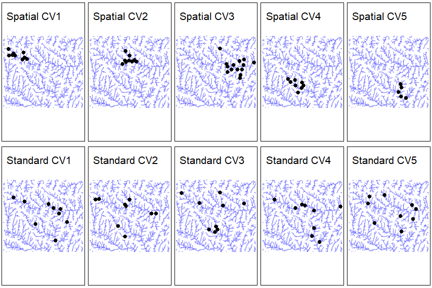
tmap_arrange(c(spatial_cv,standard_cv),ncol=5)
We see the spatial cross-validation hold-out sites cluster nicely together, whereas the standard cross-validation are randomly distributed across the region. Depending on the purpose of the model, we may favour one type of cross-validation over another.
# Setup final workflow
wf<-workflow() %>%
add_model(rf_mod) %>%
add_recipe(recip)
# Run cross-validation strategies
# tune_grid() can only work in parallel with the doParallel package
plan(sequential)
#
library(doParallel)
cl <- makeCluster(4)
registerDoParallel(cl)
set.seed(1234)
par_info<-hardhat::extract_parameter_set_dials(rf_mod) %>%
finalize(bake(prep(recip,comb_data),comb_data)) %>%
update(trees=dials::trees(range=c(20L,4000L))) # Must increase the default number of trees to get quantile predictions
final_out<-map(cv_strats,
~tune_grid(wf,
resamples=.,
metrics =metric_set(mae,rmse,rsq),
param_info = par_info,
grid=200 # Choose 200 random hyper-parameter configurations
)
)
stopCluster(cl)
# We expect the standard cross-validation to have higher accuracy than spatial
# cross-validation because the spatial autocorrelation variables should allow more accurate
# predictions from nearby sites. Conversely, the spatial cross-validation models
# show the best possible accuracy for predicting beyond the spatial extents of
# Where the data was collected.
map_dfr(final_out,show_best,5,metric = "mae",.id="Cross-validation strategy")
#> # A tibble: 10 × 10
#> Cross-validat…¹ mtry trees min_n .metric .esti…² mean n std_err .config
#> <chr> <int> <int> <int> <chr> <chr> <dbl> <int> <dbl> <chr>
#> 1 standard 63 211 6 mae standa… 2.51 5 0.249 Prepro…
#> 2 standard 102 336 14 mae standa… 2.51 5 0.245 Prepro…
#> 3 standard 88 236 8 mae standa… 2.51 5 0.229 Prepro…
#> 4 standard 71 278 14 mae standa… 2.51 5 0.230 Prepro…
#> 5 standard 58 473 12 mae standa… 2.51 5 0.246 Prepro…
#> 6 spatial 106 2713 17 mae standa… 2.56 5 0.248 Prepro…
#> 7 spatial 95 2675 19 mae standa… 2.57 5 0.246 Prepro…
#> 8 spatial 103 3843 17 mae standa… 2.57 5 0.245 Prepro…
#> 9 spatial 54 424 20 mae standa… 2.58 5 0.255 Prepro…
#> 10 spatial 80 2439 17 mae standa… 2.58 5 0.238 Prepro…
#> # … with abbreviated variable names ¹`Cross-validation strategy`, ².estimator
map_dfr(final_out,show_best,5,metric = "rsq",.id="Cross-validation strategy")
#> # A tibble: 10 × 10
#> Cross-valida…¹ mtry trees min_n .metric .esti…² mean n std_err .config
#> <chr> <int> <int> <int> <chr> <chr> <dbl> <int> <dbl> <chr>
#> 1 standard 107 1005 9 rsq standa… 0.252 5 0.108 Prepro…
#> 2 standard 102 336 14 rsq standa… 0.238 5 0.0996 Prepro…
#> 3 standard 97 2585 10 rsq standa… 0.236 5 0.0992 Prepro…
#> 4 standard 94 1990 5 rsq standa… 0.235 5 0.0986 Prepro…
#> 5 standard 1 3145 34 rsq standa… 0.235 5 0.132 Prepro…
#> 6 spatial 1 2732 8 rsq standa… 0.0940 5 0.0509 Prepro…
#> 7 spatial 2 3483 16 rsq standa… 0.0621 5 0.0254 Prepro…
#> 8 spatial 39 1600 36 rsq standa… 0.0605 2 0.0599 Prepro…
#> 9 spatial 67 1644 36 rsq standa… 0.0603 2 0.0603 Prepro…
#> 10 spatial 46 1287 36 rsq standa… 0.0597 2 0.0580 Prepro…
#> # … with abbreviated variable names ¹`Cross-validation strategy`, ².estimatorNext we build the final model. We will use the hyper-parameters that yielded the highest mean absolute error (mae) prediction accuracy using standard cross-validation. The spatial cross-validation may provide better predictions as the distance from sampled areas increases, but with so few samples, it is difficult to evaluate that aspect of the model.
# We will use mae to select best metrics overall as it is better suited
# for model selection in this context than r^2

best_tunes<-map(final_out,select_best,metric = "mae")

best_tunes
#> $standard
#> # A tibble: 1 × 4
#>    mtry trees min_n .config
#>   <int> <int> <int> <chr>
#> 1    63   211     6 Preprocessor1_Model176
#>
#> $spatial
#> # A tibble: 1 × 4
#>    mtry trees min_n .config
#>   <int> <int> <int> <chr>
#> 1   106  2713    17 Preprocessor1_Model021

# Final ranger results
final_model<-finalize_workflow(wf,best_tunes$standard) %>%
  fit(comb_data) %>%
  extract_fit_engine()

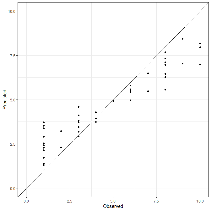
# Overall observed vs expected leaves room for improvement, but is acceptable
# given the small data size and limited predictor consideration

tibble(
  Observed=comb_data$value,
  Predicted=predict(final_model,data=bake(prep(recip),new_data=comb_data))$predictions
) %>%
  ggplot(aes(x=Observed,y=Predicted))+
  geom_point()+
  geom_abline(slope=1,intercept = 0) +
  scale_x_continuous(limits=c(0,10))+
  scale_y_continuous(limits=c(0,10))+
  theme_bw()
Finally, we will use the model to predict across the whole landscape. First we’ll assemble a table to predict from:
prediction_data<-final_attributes_all %>%
  left_join(
    # Add spatial autocorrelation variables
    hydro_out$pwise_dist %>%
      filter(origin %in% response_table$link_id) %>%
      select(origin,destination,prop_shared_catchment) %>%
      filter(origin!=destination) %>%
      rename(link_id=destination) %>%
      mutate(origin=paste0("Prop_catch_",origin)) %>%
      mutate(prop_shared_catchment=ifelse(prop_shared_catchment==1 | is.na(prop_shared_catchment),0,prop_shared_catchment)) %>%
      distinct() %>%
      filter(prop_shared_catchment!=0) %>%
      pivot_wider(names_from=origin,values_from=prop_shared_catchment,values_fill=0),
    by=c("link_id")
  ) %>%
  mutate(across(starts_with("Prop_catch_"),~ifelse(is.na(.),0,.))) %>%
  tidyr::drop_na(c(everything(),-site_id))

prediction_data
#> # A tibble: 1,196 × 140
#>    link_id site_id status   slope_lump…¹ slope…² slope…³ slope…⁴ slope…⁵ slope…⁶
#>    <chr>   <chr>   <chr>           <dbl>   <dbl>   <dbl>   <dbl>   <dbl>   <dbl>
#>  1 6       <NA>    Complete         3.93    1.90  0.178     8.26    3.97    3.25
#>  2 5       <NA>    Complete         4.73    2.43  0.385    10.4     4.85    4.56
#>  3 1202    <NA>    Complete         3.97    1.91  0.0656   12.7     4.03    3.89
#>  4 1210    <NA>    Complete         4.09    2.34  0.119    15.9     4.15    3.92
#>  5 1208    <NA>    Complete         3.58    2.21  0.0485   14.5     3.65    3.46
#>  6 1       <NA>    Complete         4.40    2.32  0.330     9.19    4.44    4.04
#>  7 1199    <NA>    Complete         3.65    2.18  0.117    12.9     3.75    3.62
#>  8 2       <NA>    Complete         3.46    1.73  0.296     8.18    3.55    3.57
#>  9 1200    <NA>    Complete         4.33    2.59  0.162    17.8     4.45    3.92
#> 10 33      <NA>    Complete         4.64    2.82  0.204    15.0     4.79    4.48
#> # … with 1,186 more rows, 131 more variables: slope_iFLO_mean <dbl>,
#> #   slope_HAiFLO_mean <dbl>, slope_HAiFLO_sd <dbl>, slope_HAiFLS_sd <dbl>,
#> #   slope_iFLO_sd <dbl>, slope_iFLS_sd <dbl>, LC_1_lumped_prop <dbl>,
#> #   LC_1_iFLS_prop <dbl>, LC_1_HAiFLS_prop <dbl>, LC_1_iFLO_prop <dbl>,
#> #   LC_1_HAiFLO_prop <dbl>, LC_2_lumped_prop <dbl>, LC_2_iFLS_prop <dbl>,
#> #   LC_2_HAiFLS_prop <dbl>, LC_2_iFLO_prop <dbl>, LC_2_HAiFLO_prop <dbl>,
#> #   LC_3_lumped_prop <dbl>, LC_3_iFLS_prop <dbl>, LC_3_HAiFLS_prop <dbl>, …
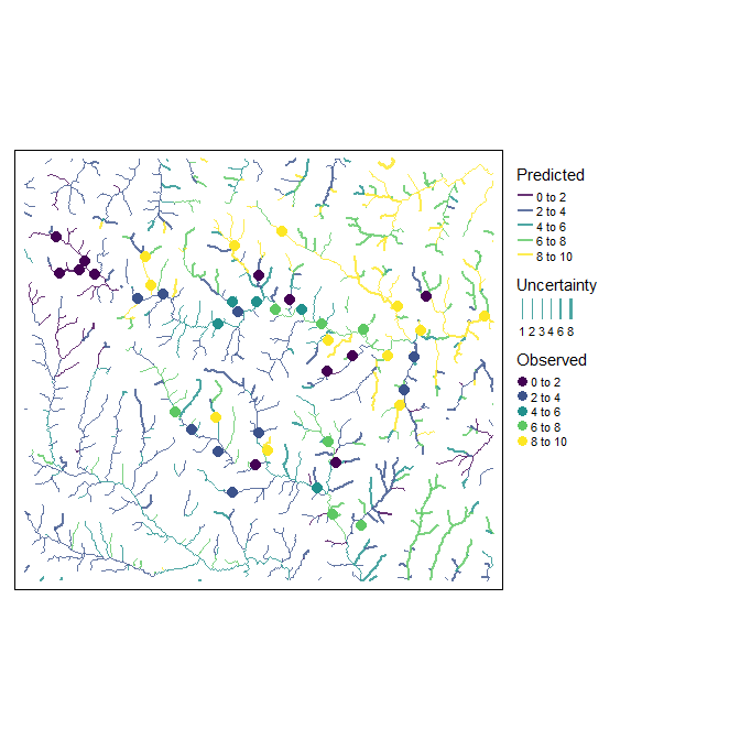
And finally, we can predict across the landscape. We’ll use the range of quantile predictions to estimate uncertainty in the model predictions. The final map we produce here shows sampled points at their measured value, stream segments are coloured according to their predicted values, and the width of the stream segment corresponds to the uncertainty in the prediction.
prediction_tbl<-tibble(
  link_id=prediction_data$link_id) %>%
  bind_cols(
    predict(final_model,
            data=bake(prep(recip),new_data=prediction_data),
            type ="quantiles",quantiles=c(0.25,0.5,0.75))$predictions %>%
      as_tibble() %>%
      setNames(c("p25","p50","p75"))
  ) %>%
  mutate(`Uncertainty` = p75-p25,
         `Predicted`=p50)

prediction_tbl
#> # A tibble: 1,196 × 6
#>    link_id   p25   p50   p75 Uncertainty Predicted
#>    <chr>   <dbl> <dbl> <dbl>       <dbl>     <dbl>
#>  1 6         1       3   5           4           3
#>  2 5         2.5     3   4           1.5         3
#>  3 1202      1       2   4           3           2
#>  4 1210      1       2   4           3           2
#>  5 1208      2       3   4           2           3
#>  6 1         3       4   6.5         3.5         4
#>  7 1199      2       3   4           2           3
#>  8 2         2       8   8           6           8
#>  9 1200      3       4   6           3           4
#> 10 33        2       3   4           2           3
#> # … with 1,186 more rows

# Since we only have predictions for entire stream segments
# This will merge and breaks in stream lines
Streams<-read_sf(hydro_out$outfile,"stream_lines") %>%
  mutate(link_id=floor(link_id)) %>%
  group_by(link_id) %>%
  summarize(geom=sf::st_union(geom)) %>%
  ungroup() %>%
  mutate(link_id=as.character(link_id))

Streams<-Streams %>%
  left_join(prediction_tbl)

Points<-read_sf(hydro_out$outfile,"snapped_points") %>%
  mutate(link_id=as.character(link_id)) %>%
  left_join(response_table %>% select(-link_id)) %>%
  filter(!is.na(link_id)) %>%
  mutate(Observed=value)

tm_shape(Streams) +
  tm_lines(col="Predicted",
           palette = "viridis",
           alpha =0.8,
           style="fixed",
           breaks =c(0,2,4,6,8,10),
           legend.show=T,
           lwd ="Uncertainty",
           scale=3) +
  tm_shape(Points) +
  tm_dots(col="Observed",
          palette = "viridis",
          legend.show=T,
          style="fixed",
          breaks =c(0,2,4,6,8,10),
          size=0.45,
          border.col="black",
          border.alpha=1,
          border.lwd=1)+
  tm_layout(legend.outside = TRUE)
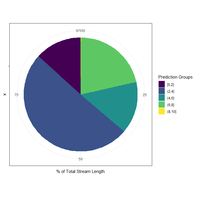
We can also summarize the percent of stream lengths that fall within predicted value classes:
Streams %>%
  mutate(strm_len=as.numeric(st_length(geom))) %>%
  as_tibble() %>%
  drop_na() %>%
  mutate(`Prediction Groups` = cut(Predicted,
                                   breaks = c(0,2,4,6,8,10),
                                   include.lowest=TRUE)
  ) %>%
  mutate(total_strm_len=sum(strm_len)) %>%
  group_by(`Prediction Groups`) %>%
  summarize(`% of Total Stream Length`=sum(strm_len)/total_strm_len*100) %>%
  distinct() %>%
  ggplot(aes(x="",y=`% of Total Stream Length`,fill=`Prediction Groups`))+
  geom_bar(width = 1, stat = "identity")+
  coord_polar("y", start=0) +
  scale_fill_viridis_d()+
  theme_bw()
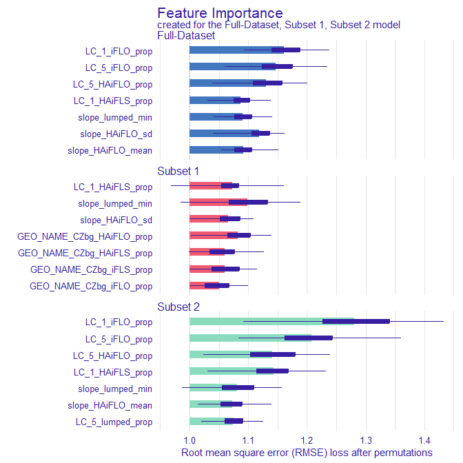
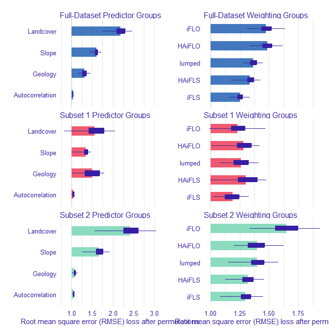
Next we will explore the final model in more detail. The DALEX package is a great tool for evaluating machine learning models. A supplemental ebook is available with great detailed examples and explanations of all the features available in this package (Biecek and Burzykowski, 2020).
# install.packages("DALEX)
library(DALEX)

# Prepare some datasets using the tidymodels recipe we specified for the model.
# We will prepare a full dataset to allow inferences about the full study region,
# as well as some spatial subsets to explore things more locally.

# Full dataset
final_data<-bake(prep(recip,comb_data),comb_data)

# One of the spatial validation folds in the upper stream
subset1_data<-assessment(cv_strats$spatial$splits[[1]])
subset1_data<-bake(prep(recip,comb_data),subset1_data)

# One of the spatial validation folds in the lower stream
subset2_data<-assessment(cv_strats$spatial$splits[[3]])
subset2_data<-bake(prep(recip,comb_data),subset2_data)

# Create some explainer objects
explainer_full <- explain(final_model,
                          data = final_data %>% select(-value),
                          y =final_data %>% select(value),
                          label = "Full-Dataset")
#> Preparation of a new explainer is initiated
#>   -> model label       :  Full-Dataset
#>   -> data              :  45  rows  109  cols
#>   -> data              :  tibble converted into a data.frame
#>   -> target variable   :  Argument 'y' was a data frame. Converted to a vector. (  WARNING  )
#>   -> target variable   :  45  values
#>   -> predict function  :  yhat.ranger  will be used (  default  )
#>   -> predicted values  :  No value for predict function target column. (  default  )
#>   -> model_info        :  package ranger , ver. 0.14.1 , task regression (  default  )
#>   -> predicted values  :  numerical, min =  1.312164 , mean =  4.608348 , max =  8.441153
#>   -> residual function :  difference between y and yhat (  default  )
#>   -> residuals         :  numerical, min =  -2.723223 , mean =  -0.03057048 , max =  3.021722
#>   A new explainer has been created!

explainer_sub1 <- explain(final_model,
                          data = subset1_data %>% select(-value),
                          y =subset1_data %>% select(value),
                          label = "Subset 1")
#> Preparation of a new explainer is initiated
#>   -> model label       :  Subset 1
#>   -> data              :  9  rows  109  cols
#>   -> data              :  tibble converted into a data.frame
#>   -> target variable   :  Argument 'y' was a data frame. Converted to a vector. (  WARNING  )
#>   -> target variable   :  9  values
#>   -> predict function  :  yhat.ranger  will be used (  default  )
#>   -> predicted values  :  No value for predict function target column. (  default  )
#>   -> model_info        :  package ranger , ver. 0.14.1 , task regression (  default  )
#>   -> predicted values  :  numerical, min =  1.312164 , mean =  3.013893 , max =  6.271169
#>   -> residual function :  difference between y and yhat (  default  )
#>   -> residuals         :  numerical, min =  -2.384044 , mean =  -0.1250044 , max =  2.434518
#>   A new explainer has been created!

explainer_sub2 <- explain(final_model,
                          data = subset2_data %>% select(-value),
                          y =subset2_data %>% select(value),
                          label = "Subset 2")
#> Preparation of a new explainer is initiated
#>   -> model label       :  Subset 2
#>   -> data              :  14  rows  109  cols
#>   -> data              :  tibble converted into a data.frame
#>   -> target variable   :  Argument 'y' was a data frame. Converted to a vector. (  WARNING  )
#>   -> target variable   :  14  values
#>   -> predict function  :  yhat.ranger  will be used (  default  )
#>   -> predicted values  :  No value for predict function target column. (  default  )
#>   -> model_info        :  package ranger , ver. 0.14.1 , task regression (  default  )
#>   -> predicted values  :  numerical, min =  2.150553 , mean =  5.80567 , max =  8.441153
#>   -> residual function :  difference between y and yhat (  default  )
#>   -> residuals         :  numerical, min =  -2.521722 , mean =  0.1943297 , max =  2.035782
#>   A new explainer has been created!

explainer_list<-list(
  `Full-Dataset`=explainer_full,
  `Subset 1`=explainer_sub1,
  `Subset 2`=explainer_sub2
)

imp_full<-lapply(explainer_list,
                 feature_importance,
                 B=100,
                 type = "ratio")
# Setting type = "ratio" means variable importance

plot(imp_full,
     max_vars = 7, # just show the top 7 predictors for each model
     bar_width =4)
The above plots show the relative importance of individual predictor variables expressed as a percent loss in model accuracy (measured as RMSE) when that variable is permuted. A greater loss in predictive accuracy implies that variable is more important in model accuracy.
As we expect, the relative importance of predictors varies depending on the region we are investigating. However, with this many predictors, it is difficult to make confident statements about the overall importance of broader groups of predictors (i.e., the relative importance of Land-cover overall vs geology; or the relative importance of local affects measured through HAIFLO vs upstream effects measured through HAIFLS). We can make these inferences by defining predictor groups.
# Define predictor variable groups
predictor_groups<-list(
  Autocorrelation = colnames(final_data)[grepl("Prop_catch_",colnames(final_data))],
  Landcover = colnames(final_data)[grepl("^LC_",colnames(final_data))],
  Geology = colnames(final_data)[grepl("^GEO_NAME_",colnames(final_data))],
  Slope = colnames(final_data)[grepl("^slope_",colnames(final_data))]
)

weighting_groups<-list(
  `lumped` = colnames(final_data)[grepl("lumped",colnames(final_data))],
  `iFLS` = colnames(final_data)[grepl("_iFLS",colnames(final_data))],
  `iFLO` = colnames(final_data)[grepl("_iFLO",colnames(final_data))],
  `HAiFLS` = colnames(final_data)[grepl("HAiFLS",colnames(final_data))],
  `HAiFLO` = colnames(final_data)[grepl("HAiFLO",colnames(final_data))]
)

imp_pred_gp<-map(explainer_list,
                 ~feature_importance(.,
                                     label=paste0(.$label," Predictor Groups"),
                                     B=100,
                                     variable_groups = predictor_groups,
                                     type = "ratio"))

imp_weighting_gp<-map(explainer_list,
                      ~feature_importance(.,
                                          label=paste0(.$label," Weighting Groups"),
                                          B=100,
                                          variable_groups = weighting_groups,
                                          type = "ratio"))

# install.packages("cowplot)

cowplot::plot_grid(
  plot(imp_pred_gp,
     bar_width =7,
     title = NULL,
     subtitle=""),
  plot(imp_weighting_gp,
     bar_width =7,
     title = NULL,
     subtitle=""),
  ncol=2
)
These plots show the relative importance of different predictors and weighting schemes for the three subsets of data.
There are many more ways to explore model results with the DALEX package, but we’ll leave that for you to explore.
This package is considered in early alpha, and bugs are expected. There is lots of room for improvements in many of the functions. The core functions may still change as the package develops and matures.
- One big area of improvement will be the handling of the output gpkg file structure.
- output gpkg may be replaced by a spatialite/rasterlite database file.
- Many functions can be cleaned and optimized further.
Kielstra, B., Mackereth, R., Melles, S., & Emilson E. (2021). hydroweight: Inverse distance-weighted rasters and landscape attributes (v1.0.0). Zenodo. https://doi.org/10.5281/zenodo.4728559
Lindsay, J.B. (2016). Whitebox GAT: A case study in geomorphometric analysis. Computers & Geosciences, 95: 75-84. https://doi.org/10.1016/j.cageo.2016.07.003
Peterson, E. E., Sheldon, F., Darnell, R., Bunn, S. E., & Harch, B. D. (2011). A comparison of spatially explicit landscape representation methods and their relationship to stream condition. Freshwater Biology, 56(3), 590–610. https://doi.org/10.1111/j.1365-2427.2010.02507.x
Przemyslaw Biecek and Tomasz Burzykowski. (2020). Explanatory Model Analysis. https://pbiecek.github.io/ema/
R Core Team (2022). R: A language and environment for statistical computing. R Foundation for Statistical Computing, Vienna, Austria. https://www.R-project.org/
Wickham, H., Bryan, J. (2021). R Packages. 2nd edition. https://r-pkgs.org/.
Wu, Q. (2020). whitebox: ‘WhiteboxTools’ R Frontend. R package version 1.4.0. https://github.com/giswqs/whiteboxR
Zimmerman, Dale L., and Jay M. Ver Hoef. (2017).”The Torgegram for fluvial variography: characterizing spatial dependence on stream networks. Journal of Computational and Graphical Statistics 26.2 253-264. https://doi.org/10.1080/10618600.2016.1247006
