Learning graph representations is a fundamental task aimed at capturing various properties of graphs in vector space. Most recent methods learn such representations for static networks. However, real world networks evolve over time and have varying dynamics. Capturing such evolution is key to predicting the properties of unseen networks. To understand how the network dynamics affect the prediction performance, various embedding approaches have been proposed. In this dynamicGEM package, we present some of the recently proposed algorithms. These algorithms include Incremental SVD, Rerun SVD, Optimal SVD, Dynamic TRIAD, Static AE, Dynamic AE, Dynamic RNN, Dynamic AERNN. We have formatted the algorithms so that they can be easily compared with each other. This library is published as DynamicGEM: A Library for Dynamic Graph Embedding Methods [0].
dynamicGEM implements the following graph embedding techniques:
- Incremental SVD: This method utilizes a perturbation matrix capturing the dynamics of the graphs along with performing additive modification on the SVD. [1]
- Rerun SVD: This method uses incremental SVD to create the dynamic graph embedding. In addition to that, it uses a tolerance threshold to restart the optimal SVD calculations and avoid deviation in incremental graph embedding. [2]
- Optimal SVD: This method decomposes adjacency matrix of the graph at each timestep using Singular Value Decomposition (SVD) to represent each node using thedlargest singular values. [3]
- Dynamic TRIAD: This method utilizes the triadic closure process to generate a graphembedding that preserves structural and evolution patterns of the graph. [4]
- Static AE: This method uses deep autoencoder to learn the representation of each node in the graph. [5]
- Dynamic AE: This method models the interconnection of nodes within and acrosstime using multiple fully connected layers. It extends Static AE for dynamic graphs. [6]
- Dynamic RNN: This method uses sparsely connected Long Short Term Memory(LSTM) networks to learn the embedding. [6]
- Dynamic AERNN: This method uses a fully connected encoder to initially ac-quire low dimensional hidden representation and feeds this representation into LSTMs to capture network dynamics. [6]
Due to variation in graph formats used by different embedding algorithms, we have written custom utils: dataprep_util which can convert various data types to the required dynamic graph format stored as list of Digraph (directed weighted graph) corresponding to the time-steps. Networkx package is used to handle these graph formats. The weight of the edges is stores as attibute "weight". The graphs are saved using nx.write_gpickle and loaded using nx.read_gpickle. For datasets that do not have these structure, we have methods (for example "get_graph_academic" for academic dataset) which can convert it into the desired graph format.
- DynamicGEM/embedding: It consists of the most recent dynamic graph embedding approaches, with each files representing a single embedding method. We also have some static graph embedding approaches as baselines.
- DynamicGEM/evaluation: Currently, we have graph reconstruction and link prediction implemented for the evaluation.
- DynamicGEM/utils: It consists of various utility functions for graph data preparation, embedding formatting, plotting utilities, etc.
- DynamicGEM/graph_generation: It constis of functions to generate dynamic stochastic block model with diminishing community.
- DynamicGEM/visualization: It consists of functions for plotting the static and dynamic embeddings of the dataset.
- DynamicGEM/experiments: The functions for hyper-paramter tuning is present in this folder.
- DynamicGEM/TIMERS: The matlab source code of the TIMERS along with added matlab modules for dataset preparation is present in this folder.
- DynamicGEM/dynamicTriad: It consists of the dynamicTriad source code.
dynamicgem is tested to work on python 3.5. The module with working dependencies are listed as follows:
- 'Cython>=0.29',
- 'tensorflow==1.11.0',
- 'h5py>=2.8.0',
- 'joblib>=0.12.5',
- 'Keras>=2.2.4',
- 'matplotlib==3.0.1',
- 'networkx>=1.11',
- 'numpy>=1.15.3',
- 'pandas>=0.23.4',
- 'scikit-learn>=0.20.0',
- 'scipy>=1.1.0',
- 'seaborn>=0.9.0',
- 'six>=1.11.0',
- 'sklearn>=0.0',
Before setting up DynamicGEM, it is suggested that the dynamic triad and TIMERS are properly set up.
- The TIMERS is originally written in matlab, in dynamicgem we have created python modules for Timers using Matlab Library Compiler. We have used Matlab R2019a to generate modules that work with python 3.5 or 3.6 . To run the matlab runtime please configure the Matlab runtime by downloading it from "https://www.mathworks.com/products/compiler/matlab-runtime.html" and following steps mentioned in "https://www.mathworks.com/help/compiler/install-the-matlab-runtime.html". The source code of TIMERS along with the setup files are located in dynamicgem/TIMERS folder.
- Do not forget to export the matlabruntime library path if you haven't used sudo to install it (i.e. sudo ./install) for Linux. For Windows, make sure the runtime library path is added in the environment Path variable.
export LD_LIBRARY_PATH="/usr/local/MATLAB/MATLAB_Runtime/v96/bin/glnxa64:/usr/local/MATLAB/MATLAB_Runtime/v96/runtime/glnxa64:/usr/local/MATLAB/MATLAB_Runtime/v96/sys/os/glnxa64:$LD_LIBRARY_PATH"
- Do not forget to export the matlabruntime library path if you haven't used sudo to install it (i.e. sudo ./install) for Linux. For Windows, make sure the runtime library path is added in the environment Path variable.
- We have build the dynamicTriad using python3. Please follow "https://github.com/luckiezhou/DynamicTriad" to install the necessary library for running the dynmicTriad. Moreover, you may build it of particular version of python as well.
- For graph_tool setup, if you are using virtual environment and not using sudo for setting up python modules, make sure to to perform following:"
    sudo find /usr/. -name graph_tool  #to find the <path-to-graph_tool> to graph)tool
    export PYTHONPATH="<path-to-graph_tool>:$PYTHONPATH"
- Also for compiled c mygraph.so module change the /dynamicGEM/dynamcigem/dynamictriad/core/gconv.py file by replacing with the absolute path of the dynamicGEM folder.
- For setting of rest of the methods, the package uses setuptools, which is a common way of installing python modules.
- To install in your home directory, use:
  export PYTHONPATH="/<...>/site-packages/:$PYTHONPATH"
  python setup.py install --user
- To install for all users on Unix/Linux:
sudo python setup.py install
- To install in your home directory, use:
import matplotlib.pyplot as plt
from time import time
import networkx as nx
import pickle
import numpy as np
import os

#import helper libraries
from dynamicgem.utils      import graph_util, plot_util, dataprep_util
from dynamicgem.evaluation import visualize_embedding as viz
from dynamicgem.visualization import plot_dynamic_sbm_embedding
from dynamicgem.evaluation import evaluate_graph_reconstruction as gr
from dynamicgem.graph_generation import dynamic_SBM_graph as sbm

#import the methods
from dynamicgem.embedding.ae_static    import AE
from dynamicgem.embedding.dynamicTriad import dynamicTriad
from dynamicgem.embedding.TIMERS       import TIMERS
from dynamicgem.embedding.dynAE        import DynAE
from dynamicgem.embedding.dynRNN       import DynRNN
from dynamicgem.embedding.dynAERNN     import DynAERNN


# Parameters for Stochastic block model graph
# Todal of 1000 nodes
node_num           = 1000
# Test with two communities
community_num      = 2
# At each iteration migrate 10 nodes from one community to the another
node_change_num    = 10
# Length of total time steps the graph will dynamically change
length             = 7
# output directory for result
outdir = './output'
intr='./intermediate'
if not os.path.exists(outdir):
    os.mkdir(outdir)
if not os.path.exists(intr):
    os.mkdir(intr)
testDataType = 'sbm_cd'
#Generate the dynamic graph
dynamic_sbm_series = list(sbm.get_community_diminish_series_v2(node_num,
                                                          community_num,
                                                          length,
                                                          1, #comminity ID to perturb
                                                          node_change_num))
graphs     = [g[0] for g in dynamic_sbm_series]
# parameters for the dynamic embedding
# dimension of the embedding
dim_emb  = 128
lookback = 2


#AE Static
embedding = AE(d            = dim_emb,
                 beta       = 5,
                 nu1        = 1e-6,
                 nu2        = 1e-6,
                 K          = 3,
                 n_units    = [500, 300, ],
                 n_iter     = 200,
                 xeta       = 1e-4,
                 n_batch    = 100,
                 modelfile  = ['./intermediate/enc_modelsbm.json',
                             './intermediate/dec_modelsbm.json'],
                 weightfile = ['./intermediate/enc_weightssbm.hdf5',
                             './intermediate/dec_weightssbm.hdf5'])
embs  = []
t1 = time()
#ae static
for temp_var in range(length):
    emb, _= embedding.learn_embeddings(graphs[temp_var])
    embs.append(emb)
print (embedding._method_name+':\n\tTraining time: %f' % (time() - t1))

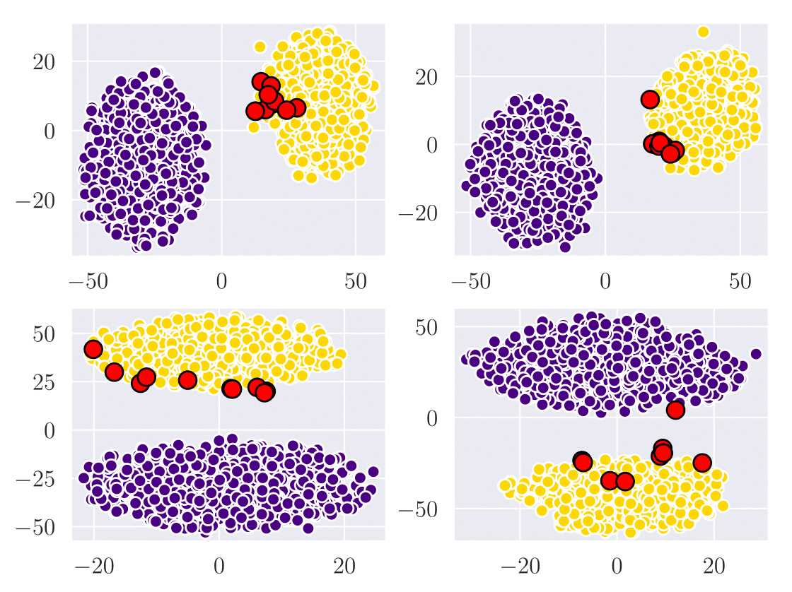
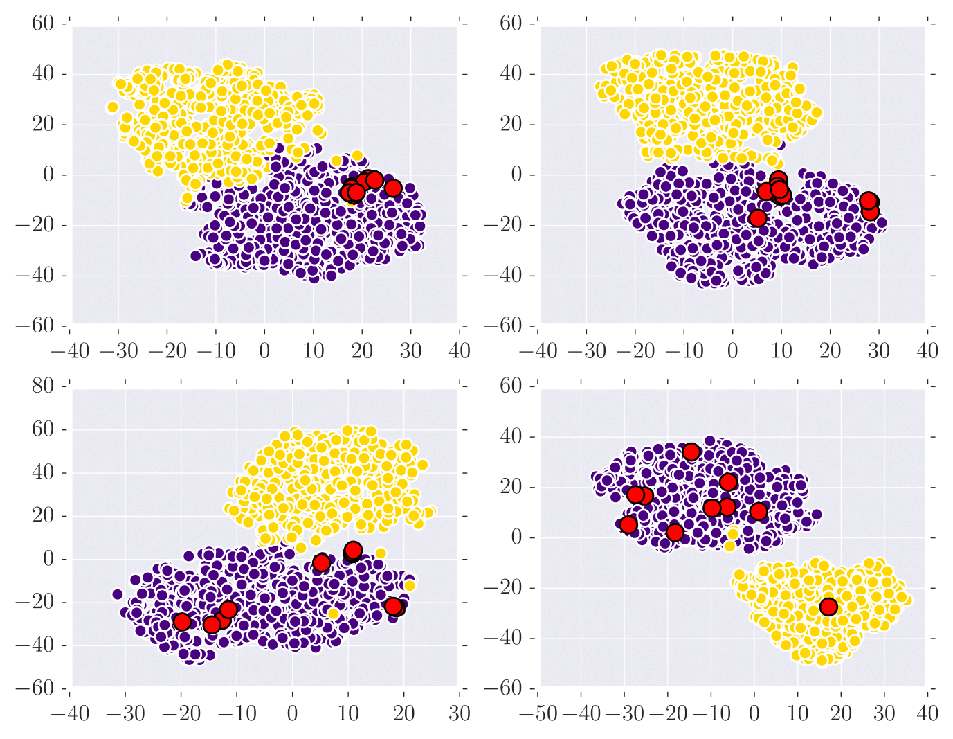
viz.plot_static_sbm_embedding(embs[-4:], dynamic_sbm_series[-4:])
The visualization of the the embedding is as follows:
#TIMERS
datafile  = dataprep_util.prep_input_TIMERS(graphs, length, testDataType)
embedding = TIMERS(K         = dim_emb,
                 Theta         = 0.5,
                 datafile      = datafile,
                 length        =  length,
                 nodemigration = node_change_num,
                 resultdir     = outdir,
                 datatype      = testDataType)
if not os.path.exists(outdir):
    os.mkdir(outdir)
outdir_tmp=outdir+'/sbm_cd'
if not os.path.exists(outdir_tmp):
    os.mkdir(outdir_tmp)
if not os.path.exists(outdir_tmp+'/incremental'):
    os.mkdir(outdir_tmp+'/incrementalSVD')
if not os.path.exists(outdir_tmp+'/rerunSVD'):
    os.mkdir(outdir_tmp+'/rerunSVD')
if not os.path.exists(outdir_tmp+'/optimalSVD'):
    os.mkdir(outdir_tmp+'/optimalSVD')

t1 = time()
embedding.learn_embedding()
embedding.get_embedding(outdir_tmp, 'optimalSVD')
print (embedding._method_name+':\n\tTraining time: %f' % (time() - t1))
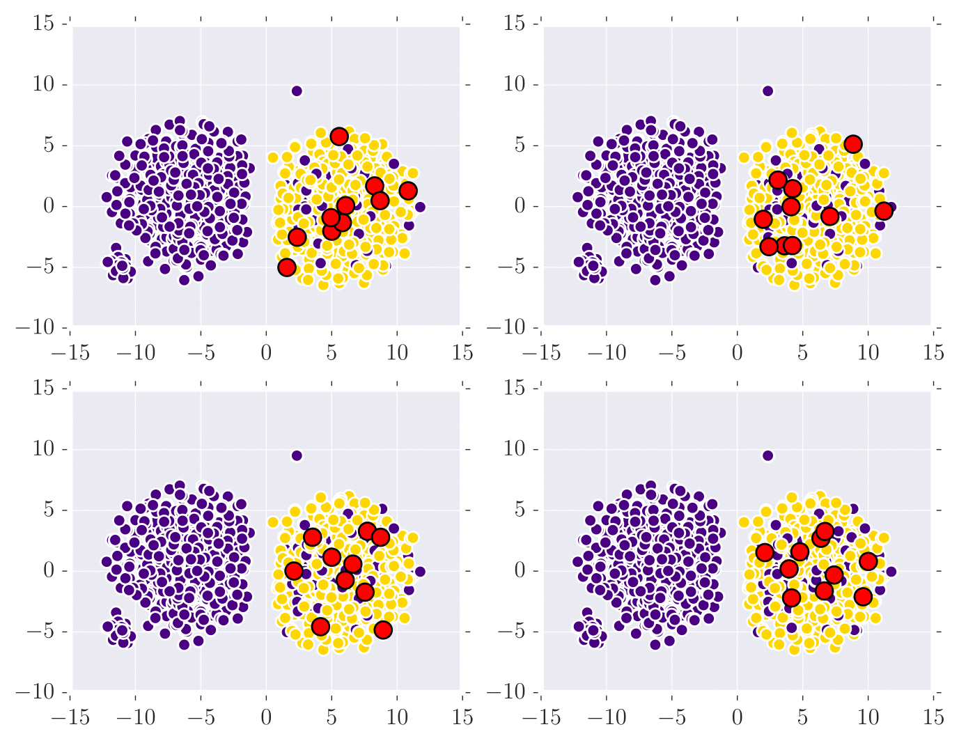
embedding.plotresults(dynamic_sbm_series)
The visualization of the the embedding is as follows:
#dynAE
embedding= DynAE(d           = dim_emb,
                 beta           = 5,
                 n_prev_graphs  = lookback,
                 nu1            = 1e-6,
                 nu2            = 1e-6,
                 n_units        = [500, 300,],
                 rho            = 0.3,
                 n_iter         = 250,
                 xeta           = 1e-4,
                 n_batch        = 100,
                 modelfile      = ['./intermediate/enc_model_dynAE.json',
                                   './intermediate/dec_model_dynAE.json'],
                 weightfile     = ['./intermediate/enc_weights_dynAE.hdf5',
                                   './intermediate/dec_weights_dynAE.hdf5'],
                 savefilesuffix = "testing" )
embs = []
t1 = time()
for temp_var in range(lookback+1, length+1):
                emb, _ = embedding.learn_embeddings(graphs[:temp_var])
                embs.append(emb)
print (embedding._method_name+':\n\tTraining time: %f' % (time() - t1))
plt.figure()
plt.clf()
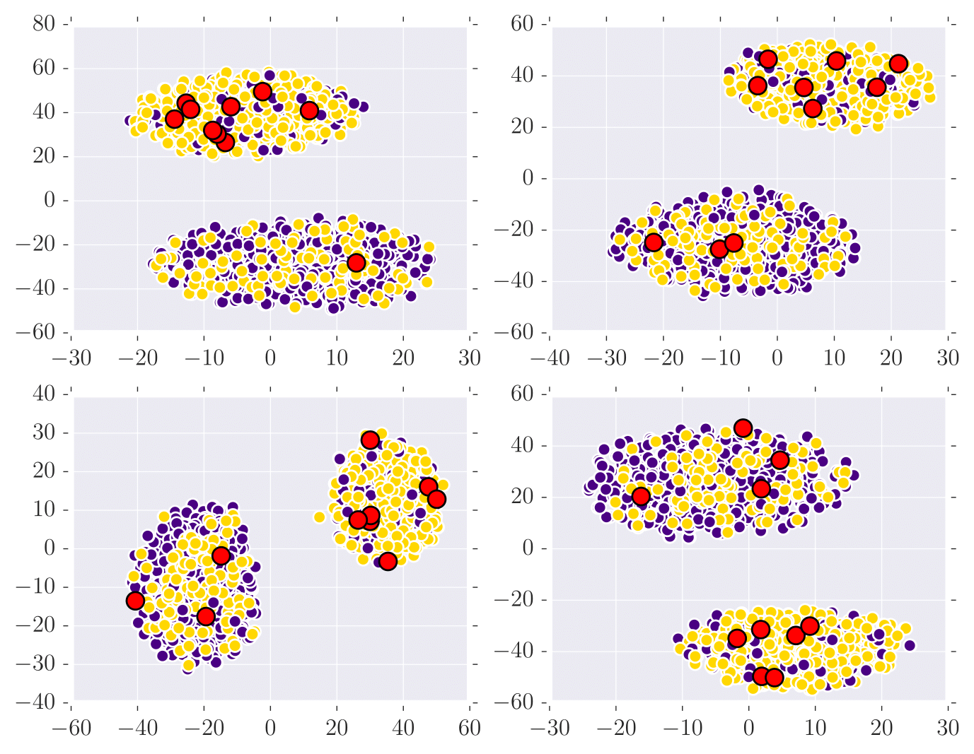
plot_dynamic_sbm_embedding.plot_dynamic_sbm_embedding_v2(embs[-5:-1], dynamic_sbm_series[-5:])
plt.show()
The visualization of the the embedding is as follows:
#dynRNN
embedding= DynRNN(d        = dim_emb,
                beta           = 5,
                n_prev_graphs  = lookback,
                nu1            = 1e-6,
                nu2            = 1e-6,
                n_enc_units    = [500,300],
                n_dec_units    = [500,300],
                rho            = 0.3,
                n_iter         = 250,
                xeta           = 1e-3,
                n_batch        = 100,
                modelfile      = ['./intermediate/enc_model_dynRNN.json',
                                  './intermediate/dec_model_dynRNN.json'],
                weightfile     = ['./intermediate/enc_weights_dynRNN.hdf5',
                                  './intermediate/dec_weights_dynRNN.hdf5'],
                savefilesuffix = "testing"  )
embs = []
t1 = time()
for temp_var in range(lookback+1, length+1):
                emb, _ = embedding.learn_embeddings(graphs[:temp_var])
                embs.append(emb)
print (embedding._method_name+':\n\tTraining time: %f' % (time() - t1))
plt.figure()
plt.clf()
plot_dynamic_sbm_embedding.plot_dynamic_sbm_embedding_v2(embs[-5:-1], dynamic_sbm_series[-5:])
plt.show()
The visualization of the the embedding is as follows:
#dynAERNN
embedding = DynAERNN(d   = dim_emb,
            beta           = 5,
            n_prev_graphs  = lookback,
            nu1            = 1e-6,
            nu2            = 1e-6,
            n_aeunits      = [500, 300],
            n_lstmunits    = [500,dim_emb],
            rho            = 0.3,
            n_iter         = 250,
            xeta           = 1e-3,
            n_batch        = 100,
            modelfile      = ['./intermediate/enc_model_dynAERNN.json',
                              './intermediate/dec_model_dynAERNN.json'],
            weightfile     = ['./intermediate/enc_weights_dynAERNN.hdf5',
                              './intermediate/dec_weights_dynAERNN.hdf5'],
            savefilesuffix = "testing")

embs = []
t1 = time()
for temp_var in range(lookback+1, length+1):
                emb, _ = embedding.learn_embeddings(graphs[:temp_var])
                embs.append(emb)
print (embedding._method_name+':\n\tTraining time: %f' % (time() - t1))
plt.figure()
plt.clf()
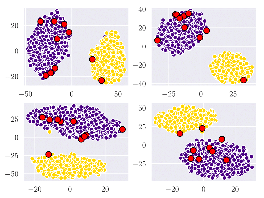
plot_dynamic_sbm_embedding.plot_dynamic_sbm_embedding_v2(embs[-5:-1], dynamic_sbm_series[-5:])
plt.show()
The visualization of the the embedding is as follows:
#dynamicTriad
datafile  = dataprep_util.prep_input_dynTriad(graphs, length, testDataType)
embedding= dynamicTriad(niters     = 20,
                 starttime  = 0,
                 datafile   = datafile,
                 batchsize  = 1000,
                 nsteps     = length,
                 embdim     = dim_emb,
                 stepsize   = 1,
                 stepstride = 1,
                 outdir     = outdir,
                 cachefn    = '/tmp/'+ testDataType,
                 lr         = 0.1,
                 beta       = [0.1,0.1],
                 negdup     = 1,
                 datasetmod = 'core.dataset.adjlist',
                 trainmod   = 'dynamicgem.dynamictriad.core.algorithm.dynamic_triad',
                 pretrain_size = length,
                 sampling_args = {},
                 validation = 'link_reconstruction',
                 datatype   = testDataType,
                 scale      = 1,
                 classifier = 'lr',
                 debug      = False,
                 test       = 'link_predict',
                 repeat     = 1,
                 resultdir  = outdir,
                 testDataType = testDataType,
                 clname       = 'lr',
                 node_num     = node_num )
t1 = time()
embedding.learn_embedding()
print (embedding._method_name+':\n\tTraining time: %f' % (time() - t1))
embedding.get_embedding()
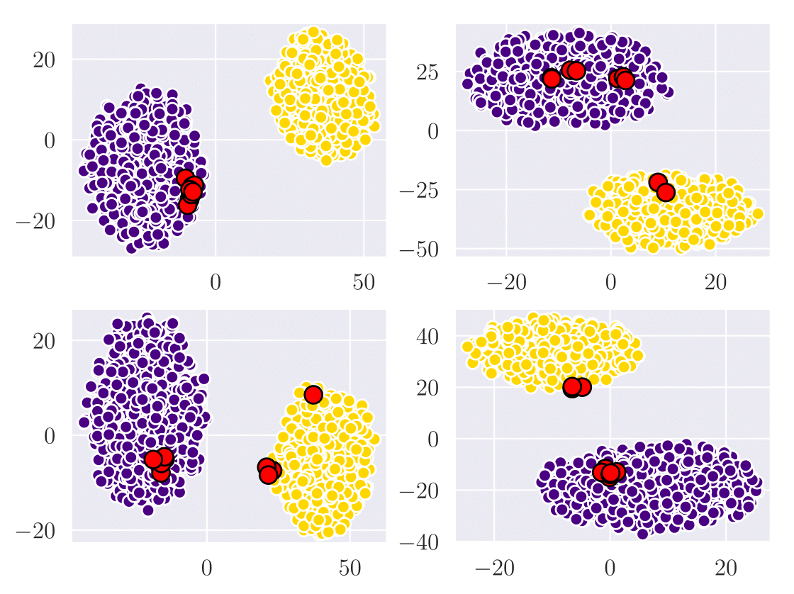
embedding.plotresults(dynamic_sbm_series)
The visualization of the the embedding is as follows:
[0] Goyal, P., Chhetri, S. R., Mehrabi, N., Ferrara, E., & Canedo, A. (2018). DynamicGEM: A Library for Dynamic Graph Embedding Methods. arXiv preprint arXiv:1811.10734.
@article{goyal2018dynamicgem,
title={DynamicGEM: A Library for Dynamic Graph Embedding Methods},
author={Goyal, Palash and Chhetri, Sujit Rokka and Mehrabi, Ninareh and Ferrara, Emilio and Canedo, Arquimedes},
journal={arXiv preprint arXiv:1811.10734},
year={2018}
}
[1] Brand, M. (2006). Fast low-rank modifications of the thin singular value decomposition. Linear algebra and its applications, 415(1), 20-30.
@article{BRAND200620,
 title = "Fast low-rank modifications of the thin singular value decomposition",
 journal = "Linear Algebra and its Applications",
 volume = "415",
 number = "1",
 pages = "20 - 30",
 year = "2006",
 note = "Special Issue on Large Scale Linear and Nonlinear Eigenvalue Problems",
 issn = "0024-3795",
 doi = "https://doi.org/10.1016/j.laa.2005.07.021",
 url = "http://www.sciencedirect.com/science/article/pii/S0024379505003812",
 author = "Matthew Brand",
 keywords = "Singular value decomposition, Sequential updating, Subspace tracking"
 }
[2] Zhang, Z., Cui, P., Pei, J., Wang, X., & Zhu, W. (2017). TIMERS: Error-Bounded SVD Restart on Dynamic Networks. arXiv preprint arXiv:1711.09541.
 @misc{zhang2017timers,
 title={TIMERS: Error-Bounded SVD Restart on Dynamic Networks},
 author={Ziwei Zhang and Peng Cui and Jian Pei and Xiao Wang and Wenwu Zhu},
 year={2017},
 eprint={1711.09541},
 archivePrefix={arXiv},
 primaryClass={cs.SI}
 }
[3] Ou, M., Cui, P., Pei, J., Zhang, Z., & Zhu, W. (2016, August). Asymmetric transitivity preserving graph embedding. In Proceedings of the 22nd ACM SIGKDD international conference on Knowledge discovery and data mining (pp. 1105-1114). ACM.
 @inproceedings{ou2016asymmetric,
 title={Asymmetric transitivity preserving graph embedding},
 author={Ou, Mingdong and Cui, Peng and Pei, Jian and Zhang, Ziwei and Zhu, Wenwu},
 booktitle={Proceedings of the 22nd ACM SIGKDD international conference on Knowledge discovery and data mining},
 pages={1105--1114},
 year={2016},
 organization={ACM}
 }
[4] Zhou, L. K., Yang, Y., Ren, X., Wu, F., & Zhuang, Y. (2018, February). Dynamic Network Embedding by Modeling Triadic Closure Process. In AAAI.
@inproceedings{zhou2018dynamic,
title={Dynamic Network Embedding by Modeling Triadic Closure Process.},
author={Zhou, Le-kui and Yang, Yang and Ren, Xiang and Wu, Fei and Zhuang, Yueting},
booktitle={AAAI},
year={2018}
}
[5] Goyal, P., Kamra, N., He, X., & Liu, Y. (2018). DynGEM: Deep Embedding Method for Dynamic Graphs. arXiv preprint arXiv:1805.11273.
@article{goyal2018dyngem,
  title={DynGEM: Deep Embedding Method for Dynamic Graphs},
  author={Goyal, Palash and Kamra, Nitin and He, Xinran and Liu, Yan},
  journal={arXiv preprint arXiv:1805.11273},
  year={2018}
}
[6] Goyal, P., Chhetri, S. R., & Canedo, A. (2018). dyngraph2vec: Capturing Network Dynamics using Dynamic Graph Representation Learning. arXiv preprint arXiv:1809.02657.
  @misc{goyal2018dyngraph2vec,
 title={dyngraph2vec: Capturing Network Dynamics using Dynamic Graph Representation Learning},
 author={Palash Goyal and Sujit Rokka Chhetri and Arquimedes Canedo},
 year={2018},
 eprint={1809.02657},
 archivePrefix={arXiv},
 primaryClass={cs.SI}
}
