Supervised Credit Risk Classification

Overview of the Analysis

The goal of this analysis is to develop a robust model capable of predicting the creditworthiness of borrowers from a peer-to-peer lending platform, and understand the main drivers of default. The model is designed to accurately differentiate between healthy loans and high-risk loans, allowing the company to minimize losses from defaulted loans while maximizing profitability by approving creditworthy borrowers.

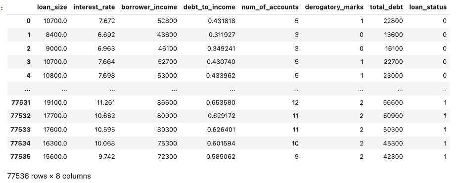
The data used in this analysis consists of historical loan records and key financial indicators that reflect the borrower's financial standing and loan attributes. These features include loan size, interest rate, borrower income, debt-to-income ratio, number of credit accounts, total debt, and the presence of derogatory marks.

The dataset includes 77,536 loan records, of which 75,036 are categorized as healthy loans, while 2,500 represent defaulted (high-risk) loans. As expected, the data is imbalanced, with a small proportion of high-risk loans, which mirrors real-world scenarios where the majority of borrowers meet their financial obligations. Advanced machine learning techniques and strategies to handle imbalanced data have been applied to mitigate this limitation.

Overview of Results

We developed and evaluated two Logistic Regression models to predict loan quality. Model 1 was trained on the original, imbalanced dataset, while Model 2 incorporated oversampling techniques to address the class imbalance. Model 2 achived an Imbalanced Binary Accuracy of 99%, above the 98% mark of model 1.

The features that more contributed to determine risk are debt-to-income-ratio, derogatory marks, and loan size.

Stages of the Machine Learning Process

The process involved in machine learning modelling consist of the following steps:

Collection and preparation of the data. This was done prior to this analysis, and the data is available this csv file. An overview of the initial dataset is shown below.

Definition of training and test data. We split the data into training and testing data sets, by applying the train_test_split function from the Model Selection module of the SciKit-learn library in Python. The training data is used to fit the model, and the test data (25% of the total set) is used to evaluate the model's predictive performance.
Creation of potencial models for evaluation. We create two Logistic Regression models using the LogisticRegression method from the Scikit-learn's Linear Model module:
- Machine Learning Model 1: this model directly uses the original loan data.
- Machine Learning Model 2: this model improves upon Model 1 by applying oversampling to address the imbalance between high-risk and healthy loans in the dataset. We used the RandomOverSampler method, from the Imblearn library, by randomly select defaulted loans (with replacement), to equalize the number of observations in both classes. The resulting class distribution is shown below.

Normalize the data. We use z-scores, so each feature has a mean of 0 and a standard deviation of 1. This step is important because it scales the variables to a comparable range, preventing features with larger magnitudes from disproportionately influencing the model’s coefficients.
Fitting of the model. We fit the training data to each model using the fit method of the Logistic Regression model. We use the default values, which are Limited-memory Broyden–Fletcher–Goldfarb–Shanno (LBFGS) for the optimization solver, and ** L2 regularization** to prevent overfitting to the training data, particularly reducing the impact of less important features.
Predicting the quality of the loans (healthy or high-risk) on the test sample data for both models. We used the predict method of the LogisticRegression model to generate this predictions.
Comparison of results. The following key metrics were used to evaluate model performance:
The precision score measures how accurately the model predicts a specific class. For example, out of loans predicted to be high-risk, what percentage were actually high-risk loans.

The recall score measures how well the model identifies a particular class. For instance, out of all actual high-risk loans, what percentage the model correctly classifies as high-risk.

The Imbalanced Binary Accuracy (IBA) measures overall accuracy. It incorporates both accuracy and the geometric mean of sensitivity (recall for the minority class) and specificity (recall for the majority class), allowing for a more balanced evaluation of classification performance.
Feature Importance. Lastly, we use SHAP analysis to identify the most influential features contributing to the model's assessment of loan health. We do this for the overall data, and individual cases.

Model Evaluation

Here are the imbalanced classification reports of both models.

The key metrics described earlier - IBA, precision, and recall— are summarized side by side for both models below.

Metric	Model 1	Model 2
Imbalanced Binary Accuracy (IBA)	98%	99%
Healthy Loans Precision	100%	100%
Healthy Loans Recall	99%	99%
High-Risk Loans Precision	84%	83%
High-Risk Loans Recall	98%	99%

The IBA shows an improvement from 98% in Model 1 to 99% in Model 2 when applying oversampling. This improvement is primarily due to same increase in the recall for hig-risk loans.

To see the specific differences, lets look into the confusion matrices of both models:

Confusion matrix for Model 1:

	Predicted Healthy Loans	Predicted High-Risk Loans
Actual Healthy Loans	18,652	113
Actual High-Risk Loans	10	609

Confusion matrix for Model 2:

	Predicted Healthy Loans	Predicted High-Risk Loans
Actual Healthy Loans	18,637	128
Actual High-Risk Loans	4	615

The incremental benefit of applying imbalance is:

Correct identification of additional 6 high-risk loans (615 - 609)
Correct identification of additional 6 healthy loans (10 - 6)

The trade off:

Missclassification of 15 healthy loans as highly risky (128 - 113)

The differences are very small. Both models are great. The user preference should determine which model to use. We will assume that, given two excellent models, avoiding default is preferable than rejecting healthy loans.

Feature Importance

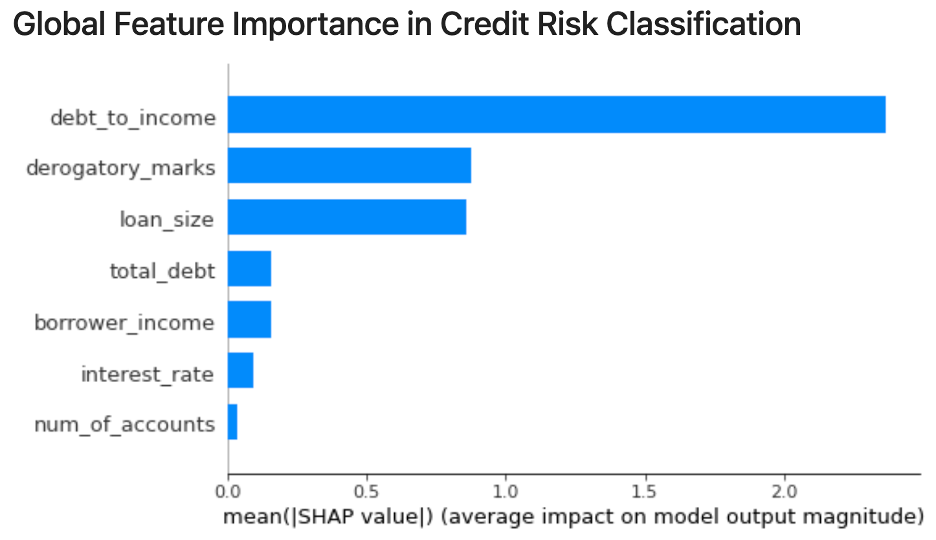
Here are the results provided by the SHAP feature importance on the overall data (see plot below):

The feature debt_to_income_ratio emerges as the most significant determinant in the model's assessment of loan performance.
derogatory_marks, followed closely by loan_size, rank as the second most important features influencing the prediction.
Features such as total_debt, borrower_income, and interest_rate play a comparatively smaller role overall, but they may become important in specific cases. These features can capture nuances in the borrower’s financial situation and provide more granular insights when the more dominant features do not fully explain the risk profile.
Lastly, number_of_accounts holds the least importance among all features, though it still contributes some value to the model's decision-making.

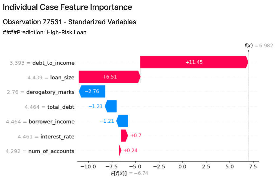
Below there is a plot for the feature contribution analysis of a high-risk individual loan prediction. Look for in deph analysis in the credit_risk_resampling notebook.

A small extract to understanding feature contributions for this individual case:

Features that Increase Risk.

High Debt-to-Income Ratio (SHAP Value = 11.45):

Starting from the base value of -6.74, the debt-to-income ratio pushes the prediction strongly toward high risk by itself. The positive SHAP value of 11.45 is a huge shift, indicating that a high debt-to-income ratio is a the main risk factor. This suggests the borrower is likely to struggle with repayment, and the model heavily penalizes such scenarios.

Large Loan Size (SHAP Value = 6.51):

Similarly, the large loan size (4+ standard deviations above average) pushes the prediction even further toward high risk, with a substantial SHAP value of 6.51. This is a dominant factor that almoves the prediction from low risk to high risk when considered alongside the debt-to-income ratio.

Conclusions:

The IBA shows an improvement from 98% in Model 1 to 99% in Model 2 when applying oversampling. This improvement is due to increase in the recall for hig-risk loans.
If we assumed that the benefit of preventing taking a bad loan is larger than the opportunity cost of not taking a good loan, then we prefer using the model 2 with the imbalance treatment, which is slighly better overall than the regular logistic model.
The features that more contributed to determine risk are debt-to-income-ratio, derogatory marks, and loan size. The other features has significantly less importance, but none has zero contribution.

Coming improvements

Since the performance of both models are pretty close, we will execute cross validation for the definitive selection of the best moodel.

Technologies Used

This project is developed in Python using JupyterLab as the interactive environment. The analysis relies heavily on the Scikit-learn (SkLearn) library, particularly the following modules:

metrics for performance evaluation
preprocessing for data preparation
model_selection for splitting data and cross-validation
linear_model for model development

Additional libraries used include:

NumPy for numerical computations
Pandas for data manipulation and analysis
shap for feature importance
imblearn for the treatment of imbalance and imbalance metrics
Pathlib for file handling
Warnings to manage warning messages in the code

Installation Guide

Clone the github repository
Install the dependencies by running: pip install -r requirements.txt in the repository directory in your terminal

Contributors

This project was created by Paola Carvajal Almeida.

Feel free to reach out via email: paola.antonieta@gmail.com

You can also view my LinkedIn profile here.

License

This project is licensed under the MIT License. This license permits the use, modification, and distribution of the code, provided that the original copyright and license notice are retained in derivative works. The license does not include a patent grant and absolves the author of any liability arising from the use of the code.

For more details, you can review the full license text in the project repository.

paocarvajal1912/Supervised_Credit_Risk_Classification