Analyse the Tetragonula bees data set in R-package prabclus. This data set gives genetic data for 236 Tetragonula (Apidae) bees from Australia and Southeast Asia. The data give pairs of alleles for 13 diploid microsatellite loci (these can be thought of as positions of genes, each characterised by two alleles). The interest here is in clustering the bees in order to find different bee species. A species is characterised by having a similar genetic makeup, whereas different species should be separated. The data set can be loaded by
library(prabclus) data(tetragonula)
In this form, the alleles are coded by numbers (every locus has a six digit number, with the first three digits referring to the first allele, and the digits 4-6 referring to the second allele). The data set needs some preprocessing in order to make it ready for work.
ta <- alleleconvert(strmatrix=tetragonula)
converts the allele codes to letters, so that each locus now has two letters (there are also some missing values coded “-”). Finally,
tai <- alleleinit(allelematrix=ta)
produces a collection of ways to represent the data (you don’t need to understand much of this; if you are curious, consult the help page of alleleinit). Particularly, tai$distmat is now a matrix of genetic distances (the help page of alleledist explains how this was computed), which is the data set you are finally asked to work with.
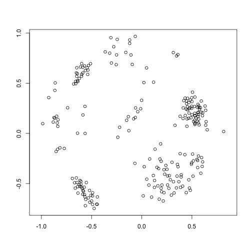
Using tai$distmat, compute an MDS and show the MDS plot. Try out different dissimilarity-based cluster analysis methods and decide which one you think is best here. Also choose a number of clusters and visualise your final clustering using the MDS. Give reasons for your choices.
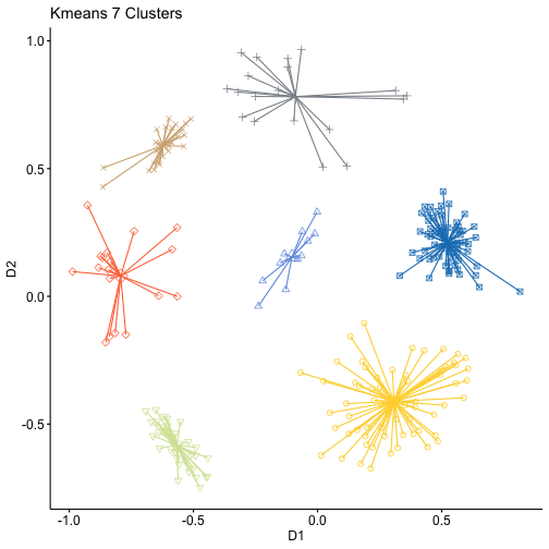
Try out the following alternative way of clustering the data: Take the points generated by the MDS and apply k-means clustering to them. Again choose a number of clusters (you may use the gap statistic for this). What are advantages and disadvantages of this approach compared to the hierarchical clustering? Do you think that this clustering is ultimately better? Do you think it would be better, for this task, to produce an MDS solution with p > 2?
data(tetragonula)

ta <- alleleconvert(strmatrix=tetragonula)
tai <- alleleinit(allelematrix=ta)

mdstai=mds(tai$distmat)


plot(mdstai$conf, xlab = "", ylab = "", asp = 1)
For this exercises I used the distances computed on the points generated by the MDS to do a better comparison with the following exercise. In a normal situation I would have used the matrix of genetic distances
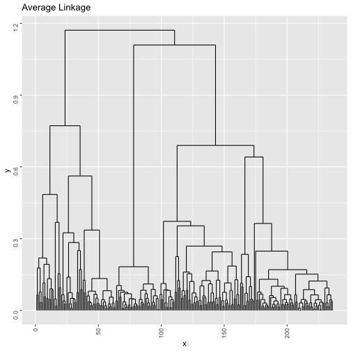
clustb <- hclust(dist(mdstai$conf),method="average")
b=ggdendrogram(clustb, rotate = F, theme_dendro = F,labels = F)
print(b + ggtitle("Average Linkage"))
tasw <- NA
tclusk <- list()
tsil <- list()
for (k in 2:30){
tclusk[[k]] <- cutree(clustb,k)
tsil[[k]] <- silhouette(tclusk[[k]],dist=dist(mdstai$conf))
tasw[k] <- summary(silhouette(tclusk[[k]],dist=dist(mdstai$conf)))$avg.width
}
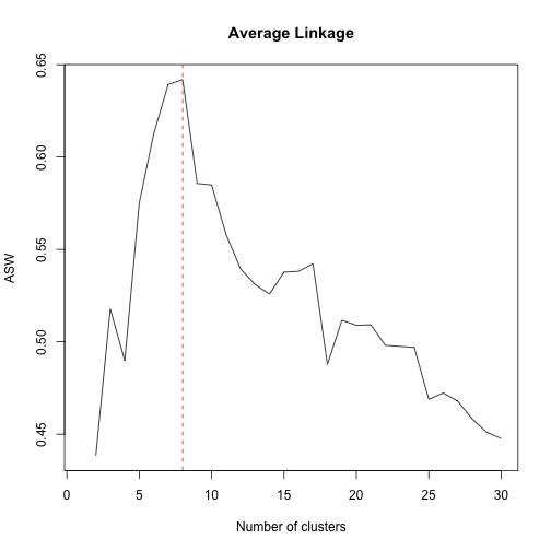
plot(1:30,tasw,type="l",xlab="Number of clusters",ylab="ASW", main="Average Linkage")
m=match(max(tasw[-1]),tasw[-1])+1
abline(v=m,col="red",lty="dashed")As we can see the suggested number of clusters is 8
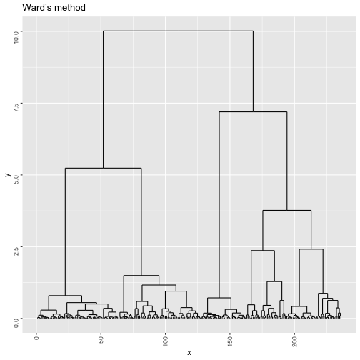
wclust <- hclust(dist(mdstai$conf),method="ward.D2")
w=ggdendrogram(wclust, rotate = F, theme_dendro = F,labels = F)
print(w + ggtitle("Ward’s method"))
tasw <- NA
tclusk <- list()
tsil <- list()
for (k in 2:30){
tclusk[[k]] <- cutree(wclust,k)
tsil[[k]] <- silhouette(tclusk[[k]],dist=dist(mdstai$conf))
tasw[k] <- summary(silhouette(tclusk[[k]],dist=dist(mdstai$conf)))$avg.width
}
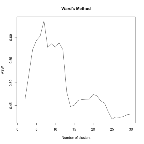
plot(1:30,tasw,type="l",xlab="Number of clusters",ylab="ASW",main="Ward's Method")
m=match(max(tasw[-1]),tasw[-1])+1
abline(v=m,col="red",lty="dashed")As we can see the suggested number of clusters is 7
pasw <- NA
pclusk <- list()
psil <- list()
for (k in 2:30){
  pclusk[[k]] <- pam(dist(mdstai$conf),k)
  # Computation of silhouettes:
  psil[[k]] <- silhouette(pclusk[[k]],dist=dist(mdstai$conf))
  # ASW needs to be extracted:
  pasw[k] <- summary(psil[[k]])$avg.width
}


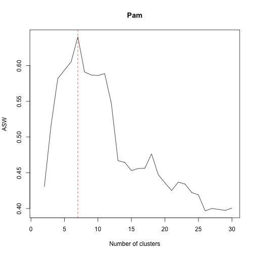
plot(1:30,pasw,type="l",xlab="Number of clusters",ylab="ASW",main="Pam")
m=match(max(pasw[-1]),pasw[-1])+1
abline(v=m,col="red",lty="dashed")
As we can see the suggested number of clusters is 8
sil<- matrix(0, nrow = 1, ncol = 3)

colnames(sil)=c("Average","Ward","Pam")
rownames(sil)=c("ASW")
sil[1,]=c( 0.6419136,0.6363861,0.6401453)
sil
## Average Ward Pam
## ASW 0.6419136 0.6363861 0.6401453
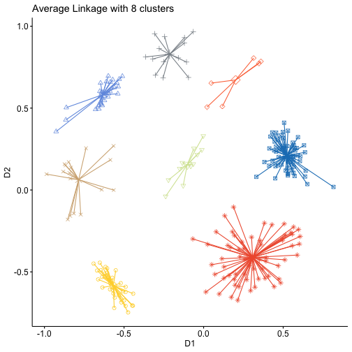
The highest value for is ASW is offered by Aveage linkage with 8 clusters, so I opted for this method.
mdstai.df=as.data.frame(mdstai$conf)
clustb10=cutree(clustb,8)

clustb10f=as.factor(clustb10)

mdstai.df= cbind(mdstai.df,clustb10f)

gg1=ggscatter( mdstai.df,
               x="D1", y="D2",
               color = "clustb10f", palette = "simpsons",
               shape = "clustb10f",
               ellipse = F,
               mean.point = TRUE,
               star.plot = TRUE)
gg1+theme(legend.position = "none")+ggtitle("Average Linkage with 8 clusters")cg1 <- clusGap(mdstai$conf,kmeans,13,B=100,d.power=2,spaceH0="scaledPCA",nstart=100)## Clustering k = 1,2,..., K.max (= 13): .. done
## Bootstrapping, b = 1,2,..., B (= 100) [one "." per sample]:
## .................................................. 50
## .........................
## Warning: did not converge in 10 iterations
## ......................... 100
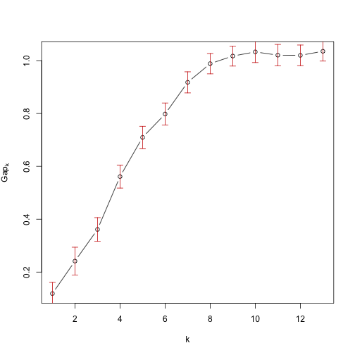
plot(cg1,main="")b=print(cg1,method="Tibs2001SEmax",SE.factor=2)## Clustering Gap statistic ["clusGap"] from call:
## clusGap(x = mdstai$conf, FUNcluster = kmeans, K.max = 13, B = 100, d.power = 2, spaceH0 = "scaledPCA", nstart = 100)
## B=100 simulated reference sets, k = 1..13; spaceH0="scaledPCA"
## --> Number of clusters (method 'Tibs2001SEmax', SE.factor=2): 7
## logW E.logW gap SE.sim
## [1,] 4.0022215 4.120870 0.1186486 0.04227843
## [2,] 3.3679534 3.609483 0.2415292 0.05252593
## [3,] 2.7732498 3.134459 0.3612093 0.04485499
## [4,] 2.1526272 2.713858 0.5612306 0.04357457
## [5,] 1.8003177 2.509855 0.7095375 0.04182651
## [6,] 1.5158069 2.313790 0.7979829 0.04162255
## [7,] 1.2160338 2.133873 0.9178394 0.03987527
## [8,] 0.9815963 1.970144 0.9885474 0.03848105
## [9,] 0.8133341 1.830623 1.0172891 0.03772344
## [10,] 0.6778002 1.710782 1.0329813 0.04013155
## [11,] 0.5806698 1.601325 1.0206549 0.04057282
## [12,] 0.4771784 1.497111 1.0199325 0.03909452
## [13,] 0.3640966 1.399467 1.0353706 0.03687262
The suggested number of clusters suggested by "Tibs2001SEmax" is 7
kmeans=kmeans(mdstai$conf,7,nstart=100)
km=as.factor(kmeans$cluster)

mdstai.df= cbind(mdstai.df,km)
gg1=ggscatter( mdstai.df,
               x="D1", y="D2",
               color = "km", palette = "simpsons",
               shape = "km",
               ellipse = F,
               mean.point = TRUE,
               star.plot = TRUE)
gg1+theme(legend.position = "none")+ggtitle("Kmeans 7 Clusters")adjustedRandIndex(kmeans$cluster,clustb10)## [1] 0.9851412
In this case it's very hard to tell wich one of the two solutions is better, they look identical and this is confirmed by an ARI almost equal to 1. More generarly we can say that kmeans is less computational demanding but its performance depends on the validity of the assumptions at its base. The results also depend on on the starting centroids, so we can say that it's affected by randomness and we get a local optimum not a global one. One crucial point is also the choice of k that happens before the algorithm is computed, not after like in the case of hierarchical clustering, so the results are affected also by this. Hierarchical clustering is also more flexible because it useses dissimilarities, so we can include also cathegorical variables.
I don't think that in this case it would be better to consider p>2 because the clusters can be identified pretty clearly using the graphical reprsentation.
