On the Virtuale page of the course (under Data Sets) you find the dataset baseball.txt. You can read it using baseball <- read.csv("baseball.txt",header=TRUE) The baseball dataset contains salary information for 337 Major League Baseball (MLB) players who are not pitchers and played at least one game during both the 1991 and 1992 seasons. The purpose of the study is to determine whether a baseball player’s salary is a reflection of his offensive performance. A good predictive performance is also of interest. For each player, the salary from the 1992 season along with 12 offensive statistics from the 1991 season were collected. In addition to these variables, there are 4 indicator variables which identify free agency and eligibility for arbitration.
Find an appropriate linear regression model explaining the response variable y by some or all of the other variables. Interpret your final model, and comment on the appropriateness of the model assumptions. It may be useful to transform the y-variable. As part of your analyses, compare at leats one model that uses the original y-variable and one model that uses a transformed y-variable using a cross-validation scheme that makes models with and without transformation appropriately comparable.
For the baseball dataset above (with untransformed y) run backward elimination using the regsubsets-function, and compare the models with different numbers of variables by estimated expected prediction errors1 using LOO-CV, 5-fold, and 10-fold CV. Compare the different prediction error estimates, and the rankings of models according to the three CV-schemes. To what extent do they agree with each other?
For the Ozone data, use “outer” cross-validation (you can use LOO-CV, 5-fold, or 10-fold as you like) to compare the full model, and the models selected by backward elimination, forward selection, and best subset selection regarding the estimated expected prediction error in a way that is unaffected by selection bias (this means double crossvalidation if cross-validation is used to select the model in an “inner loop”, but if the model is selected by AIC or fixed, only “outer” cross-validation of the full selection process is needed). Does the result differ from the result given on the slides without using double cross-validation? Also save all numbers of variables that were chosen by backward, forward, and best subset selection on the different datasets that occur in the outer CV, and comment on the stability of these selections.
library(MASS)
library(plyr)
library(MLmetrics)
library(leaps)
library(knitr)
baseball <-read.csv("baseball.txt",header=TRUE)
varnames <-names(baseball)[-1]
response <-names(baseball)[1]
unicef.full.model <-as.formula(paste(response,"~",paste(varnames,collapse=" + ")))
fullmod=lm(unicef.full.model,data = baseball)
empty <-lm(baseball$y~1,data=baseball)
backward=step(fullmod,direction="backward", data=unicef,trace=0)
forward=step(empty,direction="forward",scope=unicef.full.model, data=unicef,trace = 0)

best=lm(y ~ x3 + x7 + x8 + x10 + x11 + x12 + x13 + x14 + x15, data=baseball)
summary(best)
##
## Call:
## lm(formula = y ~ x3 + x7 + x8 + x10 + x11 + x12 + x13 + x14 +
## x15, data = baseball)
##
## Residuals:
## Min 1Q Median 3Q Max
## -1897.9 -460.6 18.3 346.9 3252.8
##
## Coefficients:
## Estimate Std. Error t value Pr(>|t|)
## (Intercept) -111.046 89.033 -1.247 0.2132
## x3 5.782 3.224 1.794 0.0738 .
## x7 24.026 9.762 2.461 0.0144 *
## x8 16.031 3.820 4.196 3.50e-05 ***
## x10 -9.338 1.881 -4.964 1.11e-06 ***
## x11 11.516 4.507 2.555 0.0111 *
## x12 -10.110 7.239 -1.397 0.1635
## x13 1363.764 104.209 13.087 < 2e-16 ***
## x14 -276.567 136.902 -2.020 0.0442 *
## x15 819.485 111.805 7.330 1.82e-12 ***
## ---
## Signif. codes: 0 '***' 0.001 '**' 0.01 '*' 0.05 '.' 0.1 ' ' 1
##
## Residual standard error: 693.3 on 327 degrees of freedom
## Multiple R-squared: 0.6958, Adjusted R-squared: 0.6874
## F-statistic: 83.1 on 9 and 327 DF, p-value: < 2.2e-16
Both backward and forward selection agree on choosing the followig model as best one: y ~ x3 + x7 + x8 + x10 + x11 + x12 + x13 + x14 + x15
The results in terms of adjusted R-squared are convincing, an high proportion of the variance of the dependent variable is explained by the model. Most of the coefficiets related to the variables are significant for an
par(mfrow=c(2,2))
plot(best,1)
plot(best,2)
plot(best,3)
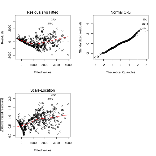
The scale-loatio plot highlights a pattern between the two variables, so we are in the case of heteroschedasticity. We can solve this problem exploiting the Box-Cox transformation.
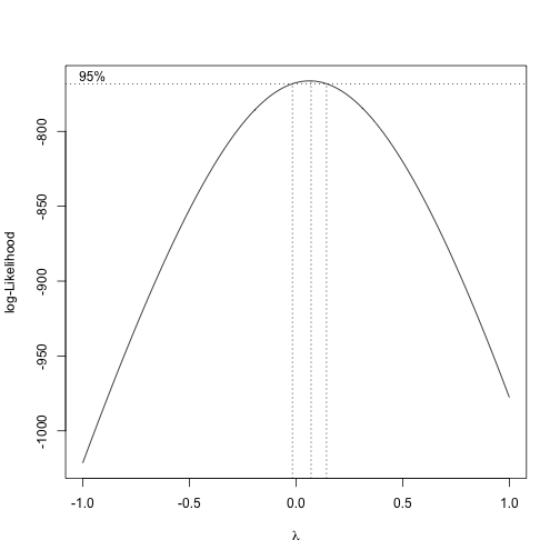
box_cox <- boxcox(best, lambda = seq(-1,1, by=.1), main = "Box-Cox Power Transformation")The graph suggests a value for
best_log=lm(log(y) ~ x3 + x7 + x8 + x10 + x11 + x12 + x13 + x14 + x15, data=baseball)
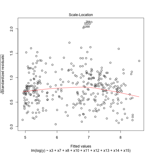
plot(best_log,3)
Now the heteroschedasticity problem seem to be solved
n=337
yhat <- numeric(0)
yhat_log= numeric(0)
for (i in 1:n){
  bs <- lm(y ~ x3 + x7 + x8 + x10 + x11 + x12 + x13 + x14 + x15, data=baseball[-i,])
  yhat[i] <- predict(bs,baseball[i,])
  bs_log=lm(log(y) ~ x3 + x7 + x8 + x10 + x11 + x12 + x13 + x14 + x15, data=baseball[-i,])
  mse=sum(bs_log$residuals^2)/bs_log$df.residual
  yhat_log[i] <- exp(predict(bs_log,baseball[i,]))*exp(mse*0.5)

}
sqloss <- sqrt(mean((yhat-baseball$y)^2))
sqloss_log <- sqrt(mean((yhat_log-baseball$y)^2))

trial <-matrix(c(sqloss,sqloss_log), ncol=2,nrow = 1)
colnames(trial) <-c("y","log(y)")
rownames(trial) <-c("sqlossfunction")
kable(trial)| y | log(y) | |
|---|---|---|
| sqlossfunction | 711.9639 | 724.9453 |
P=16
n=337
bestsub <- regsubsets(unicef.full.model,data=baseball,nvmax=16,method="exhaustive")
sbest <- summary(bestsub)

sqrlossbest_LOO <- numeric(0)
yhat_LOO <- matrix(NA,nrow=P,ncol=n)
modfor <- list()

for (j in 1:P){
  modfor[[j]] <-as.formula(paste(response,"~",paste(varnames[sbest$which[j,2:(P+1)]],
                                                    collapse=" + ")))
}
for (j in 1:P){
  for (i in 1:n){
    fmi <- lm(modfor[[j]], data=baseball[-i,])
    yhat_LOO[j,i] <- predict(fmi,baseball[i,])
  }
  sqrlossbest_LOO[j] <- sqrt(mean((yhat_LOO[j,]-baseball$y)^2))
}


###10-fold

#random shuffle data
baseball_shuff<-baseball[sample(nrow(baseball)),]

#Create 10 equally size folds
indexes <- cut(seq(1,nrow(baseball_shuff)),breaks=10,labels=FALSE)
Indexes=list()
for(i in 1:10){
  Indexes[[i]] <- which(indexes==i,arr.ind=TRUE)

}


sqrlossbest_10F <- numeric(0)
yhat_10F <- matrix(NA,nrow=P,ncol=n)
for (j in 1:P){
  for (i in 1:10){
    fmi <- lm(modfor[[j]], data=baseball_shuff[-Indexes[[i]],])
    yhat_10F[j,Indexes[[i]]] <- predict(fmi,baseball_shuff[Indexes[[i]],])
  }
  sqrlossbest_10F[j] <- sqrt(mean((yhat_10F[j,]-baseball_shuff$y)^2))
}


#5 Fold cv
baseball_shuff<-baseball[sample(nrow(baseball)),]

#Create 10 equally size folds
indexes <- cut(seq(1,nrow(baseball_shuff)),breaks=5,labels=FALSE)
Indexes=list()
for(i in 1:5){
  Indexes[[i]] <- which(indexes==i,arr.ind=TRUE)

}


sqrlossbest_5F <- numeric(0)
yhat_5F <- matrix(NA,nrow=P,ncol=n)
for (j in 1:P){
  for (i in 1:5){
    fmi <- lm(modfor[[j]], data=baseball_shuff[-Indexes[[i]],])
    yhat_5F[j,Indexes[[i]]] <- predict(fmi,baseball_shuff[Indexes[[i]],])
  }
  sqrlossbest_5F[j] <- sqrt(mean((yhat_5F[j,]-baseball_shuff$y)^2))
}

trial <-matrix(round(c(sqrlossbest_LOO,sqrlossbest_10F,sqrlossbest_5F),1), ncol=16,nrow = 3,dimnames=list(c("LOO","10-Folds","5-Folds"),rep("",P)))
trial
##
## LOO 927.6 734.5 711.2 714.2 718.4 727.0 743.4 712.2 711.7 713.0 722.7 810.7 728.3
## 10-Folds 803.4 719.5 711.6 714.8 719.4 928.4 734.5 710.3 713.3 717.3 726.2 753.0 724.6
## 5-Folds 745.0 712.5 713.9 715.6 722.9 801.6 719.0 711.2 716.4 718.2 926.8 744.0 724.8
##
## LOO 723.0 737.6 743.2
## 10-Folds 734.3 740.7 744.8
## 5-Folds 738.0 743.1 753.1
trial <-matrix(c(order(sqrlossbest_LOO),order(sqrlossbest_10F),order(sqrlossbest_5F)),ncol=16,nrow=3)
rownames(trial) <-c("LOO","10-Fold cv","5-Fold cv" )
kable(trial)
## Warning in kable_markdown(x = structure(c("LOO", "10-Fold cv", "5-Fold cv", : The table
## should have a header (column names)
| LOO | 7 | 9 | 12 | 5 | 4 | 1 | 9 | 10 | 14 | 16 | 2 | 6 | 9 | 12 | 4 | 16 |
| 10-Fold cv | 8 | 10 | 13 | 15 | 3 | 7 | 6 | 11 | 5 | 4 | 1 | 7 | 11 | 13 | 15 | 2 |
| 5-Fold cv | 6 | 11 | 14 | 16 | 2 | 8 | 12 | 13 | 15 | 3 | 8 | 5 | 10 | 14 | 3 | 1 |
In this table it's showcasedthe rankings of models according to the three CV-schemes in descending order
ozone=read.table("ozone.txt",header = T)
ozone<-ozone[complete.cases(ozone),]
varnames <- c("ALTER", "ADHEU", "SEX", "HOCHOZON", "AMATOP", "AVATOP",
              "ADEKZ", "ARAUCH", "AGEBGEW", "FSNIGHT", "FLGROSS",
              "FMILB", "FNOH24", "FTIER", "FPOLL", "FLTOTMED", "FO3H24",
              "FSPT", "FTEH24", "FSATEM", "FSAUGE", "FLGEW", "FSPFEI",
              "FSHLAUF")
response <- "FFVC"

ozone<-ozone[sample(nrow(ozone)),]
indexes <- cut(seq(1,nrow(ozone)),breaks=10,labels=FALSE)
fold=list()
for(i in 1:10){
  fold[[i]] <- which(indexes==i,arr.ind=TRUE)

}

# inner loop could be different - can also do LOO or 5-fold in inner loop.
nmodels <- 24 # That should be enough...

response <- 1
cvdata <- ozone
names(cvdata)[response] <- "y"
full.model=as.formula(paste("y","~", paste(varnames,collapse=" + ")))
n=496
yhat <- besti <- numeric(0)
fmbesti <- mbesti <- bestmodel <- modforcvi <- list()
yhati <- sqrlossi <- matrix(NA,nrow=nmodels,ncol=n)
foldnumber=10
for (i in 1:foldnumber){
  cat("Outer fold ",i,"\n")
  yhati <- matrix(NA,nrow=nmodels,ncol=n)
  modforcv <- list()
  for (j in (1:foldnumber)[-i]){
    cat("Inner fold ",j,"\n")
    bestsubi <- regsubsets(full.model,data=cvdata[-c(fold[[i]],fold[[j]]),],
                           nvmax=nmodels,method="forward") # leaving folds i and j out
    sbesti <- summary(bestsubi)
    for (k in 1:nmodels){
      modforcv[[k]] <- as.formula(paste("y~", paste(varnames[sbesti$which[k,2:(P+1)]],
                                                    collapse=" + "))) # extract best model
      fmi <- lm(modforcv[[k]], data=cvdata[-c(fold[[i]],fold[[j]]),]) # fit it
      yhati[k,fold[[j]]] <- predict(fmi,cvdata[fold[[j]],])
      # predict fold j for finding best k
    } # end for k (models)
 } # end for j (inner loop) outer loop still running
  for (k in 1:nmodels)
    sqrlossi[k,i] <- sqrt(mean((yhati[k,]-cvdata$y)^2,na.rm=TRUE))
  besti[i] <- which.min(sqrlossi[,i]) # Best model chosen without fold i
  bestmodel[[i]] <- regsubsets(full.model,data=cvdata[-fold[[i]],],
                               nvmax=besti[i],method="forward") # run forward selection on data without fold i
  sbesti <- summary(bestmodel[[i]])
  modforcvi[[i]] <- as.formula(paste("y~", paste(varnames[sbesti$which[besti[[i]],2:(P+1)]],
                                                 collapse=" + ")))
  # Extract best model as found in inner loop
  fmbesti[[i]] <- lm(modforcvi[[i]], data=cvdata[-fold[[i]],]) # Fit this
  yhat[fold[[i]]] <- predict(fmbesti[[i]],cvdata[fold[[i]],])
  # Predict fold i data with best model selected without fold i.
}
sqrlossbest <- sqrt(mean((yhat-cvdata$y)^2))
besti


yhat <- numeric(0)
lmodel <- list()
besti_2=c()
for (i in 1:foldnumber){
  cat("Leave out ",i,"\n")
  empty <- lm(y~1,data=cvdata[-fold[[i]],])
  lmodel[[i]] <- step(empty,scope=full.model,direction="forward",
                      data=cvdata[-fold[[i]],],trace=0)

  yhat[fold[[i]]] <- predict(lmodel[[i]],cvdata[fold[[i]],])
  besti_2[i]=dim(lmodel[[i]][["model"]])[2]-1
}
sqrlossforward <- sqrt(mean((yhat-cvdata$y)^2))

yhat <- numeric(0)
lmodel <- list()
besti_3=c()
for (i in 1:foldnumber){
  cat("Leave out ",i,"\n")
  fullmod <- lm(full.model, data=cvdata[-fold[[i]],])
  lmodel[[i]] <- step(fullmod,direction="backward",
                      data=cvdata[-fold[[i]],],trace = 0)
  yhat[fold[[i]]] <- predict(lmodel[[i]],cvdata[fold[[i]],])
  besti_3[i]=dim(lmodel[[i]][["model"]])[2]-1

}
sqrlossbackward <- sqrt(mean((yhat-cvdata$y)^2))| best subset | forward | backward |
|---|---|---|
| 0.2159978 | 0.2179183 | 0.2174766 |
| best subset | 22 | 20 | 23 | 24 | 12 | 10 | 9 | 10 | 11 | 12 |
| forward | 22 | 21 | 21 | 8 | 13 | 9 | 10 | 12 | 12 | 11 |
| backward | 24 | 24 | 22 | 8 | 11 | 10 | 8 | 13 | 12 | 11 |
With the three methods we don't always get the same number of variables inserted in the model, nevertheless the results seem pretty stable being pretty close to each other. Forward and backward selection give similar results, the best subset tends to insert far too many variables in the model.


