parth-20-07/Sliding-Mode-Control-Based-3D-Trajectory-Tracking-for-UAVs

The aim of the project is to design and implement various forms of trajectory controllers for Quadcopter

Table of Contents

• Introduction
• Setup the environment
  • Install ROS1 Noetic
  • Setup Crazyflie 2.0 Quadrotor in Gazebo
• Dynamic Model
• Problem Statement
  • Part 1: Trajectory Generation
  • Part 2: Controller Design
    • Designing Controller 1 to control z
    • Designing Controller 2 to control phi
    • Designing Controller 3 to control theta
    • Designing Controller 4 to control psi
    • Tuning parameters
  • Part 3: Programming the Controllers
    • Fetching the current drone parameters
    • Controller 1
    • Controller 2
    • Controller 3
    • Controller 4
    • Saturation Function
    • Allocation Matrix
    • Limiting Rotor Velocity
    • Calculating Omega
    • Publishing the Rotor Values to topic
  • Part 4: Plotting the system performance
    • Saving System Data into Array
    • Performance Visualization
  • Part 5: Performance Testing in Gazebo
• Packages used
• Design Details
• License

Introduction

The objective of this project is to develop a robust control scheme to enable a quadrotor to track desired trajectories in the presence of external disturbances.

The control design under study will be tested on the Crazyflie 2.0 platform. Crazyflie is a quadrotor that is classified as a micro air vehicle (MAV), as it only weighs 27 grams and can fit in your hand. The size makes it ideal for flying inside a lab without trashing half the interior. Even though the propellers spin at high RPMs, they are soft and the torque in the motors is very low when compared to a brushless motor, making it relatively crash tolerant. The Crazyflie 2.0 features four 7mm coreless DC-motors that give the Crazyflie a maximum takeoff weight of 42g.

The Crazyflie 2.0 is an open source project, with source code and hardware design both documented and available. For more information, see the link below: https://www.bitcraze.io/products/old-products/crazyflie-2-0/

Crazyflie 2.0 Quadrotor Hardware

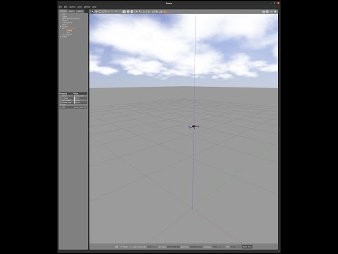
Crazyflie 2.0 Quadrotor Gazebo Simulation

Note: The Complete project is build and tested on Ubuntu 20.04LTS with ROS Noetic and not tested on any other system. Kindly proceed with caution and loads of google usage for porting it to any other system. And as always, common sense is must before anything!!

Setup the environment

Install ROS1 Noetic

1. Setup your sources.list Setup your computer to accept software from packages.ros.org.

   sudo sh -c 'echo "deb http://packages.ros.org/ros/ubuntu $(lsb_release -sc) main" > /etc/apt/sources.list.d/ros-latest.list'
   

2. Set up your keys

   sudo apt install curl # if you haven't already installed curl
   curl -s https://raw.githubusercontent.com/ros/rosdistro/master/ros.asc | sudo apt-key add -
   

3. Installation First, make sure your Debian package index is up-to-date:

   sudo apt update
   

   Desktop-Full Install: (Recommended) : Everything in Desktop plus 2D/3D simulators and 2D/3D perception packages

   sudo apt install ros-noetic-desktop-full
   

4. Environment setup You must source this script in every bash terminal you use ROS in.

   source /opt/ros/noetic/setup.bash
   

   It can be convenient to automatically source this script every time a new shell is launched. These commands will do that for you.

   echo "source /opt/ros/noetic/setup.bash" >> ~/.bashrc
   source ~/.bashrc
   

5. Dependencies for building packages Up to now you have installed what you need to run the core ROS packages. To create and manage your own ROS workspaces, there are various tools and requirements that are distributed separately. For example, rosinstall is a frequently used command-line tool that enables you to easily download many source trees for ROS packages with one command.

   To install this tool and other dependencies for building ROS packages, run:

   sudo apt install python3-rosdep python3-rosinstall python3-rosinstall-generator python3-wstool build-essential
   

   Initialize rosdep

   Before you can use many ROS tools, you will need to initialize rosdep. rosdep enables you to easily install system dependencies for source you want to compile and is required to run some core components in ROS. If you have not yet installed rosdep, do so as follows.

   sudo apt install python3-rosdep
   

   With the following, you can initialize rosdep.

   sudo rosdep init
   rosdep update
   

6. Create a workspace

   mkdir -p ~/rbe502_ros/src
   cd ~/rbe502_ros
   catkin_make
   echo "source ~/rbe502_ros/devel/setup.bash" >> ~/.bashrc
   source ~/rbe502_ros/devel/setup.bash
   

7. Install the Control and Effort Dependencies for Gazebo

   sudo apt-get update
   sudo apt-get upgrade
   sudo apt update
   sudo apt-get install ros-noetic-ros-control ros-noetic-ros-controllers
   sudo apt-get install ros-noetic-gazebo-ros-pkgs ros-noetic-gazebo-ros-control
   

8. With all dependencies ready, we can build the ROS package by the following commands.

   cd ~/rbe502_ros
   catkin_make
   

Setup Crazyflie 2.0 Quadrotor in Gazebo

To set up the Crazyflie 2.0 quadrotor in Gazebo, we need to install additional ROS dependencies for building packages as below:

sudo apt update
sudo apt install ros-noetic-joy ros-noetic-octomap-ros ros-noetic-mavlink
sudo apt install ros-noetic-octomap-mapping ros-noetic-control-toolbox
sudo apt install python3-vcstool python3-catkin-tools protobuf-compiler libgoogle-glog-dev
rosdep update
sudo apt-get install ros-noetic-ros libgoogle-glog-dev

We are now ready to create a new ROS workspace and download the ROS packages for the robot:

mkdir -p ~/rbe502_project/src
cd ~/rbe502_project/src
catkin_init_workspace # initialize your catkin workspace
cd ~/rbe502_project
catkin init
catkin build -j1
cd ~/rbe502_project/src
git clone -b dev/ros-noetic https://github.com/gsilano/CrazyS.git
git clone -b med18_gazebo9 https://github.com/gsilano/mav_comm.git

Note: a new ROS workspace is needed for the project, because the CrazyS Gazebo package is built using the catkin build tool, instead of catkin_make.

Note: -j1 in catkin build is for safety so it does not cause you computer to hang. It makes your code to build on just one core. Slow but ensures it compiles without issues

We need to build the project workspace using python_catkin_tools , therefore we need to configure it:

cd ~/rbe502_project
rosdep install --from-paths src -i
rosdep update
catkin config --cmake-args -DCMAKE_BUILD_TYPE=Release -DCATKIN_ENABLE_TESTING=False
catkin build -j1

This is gonna take a lot of time. Like a real lot. So maybe make yourself a cup of coffee meanwhile? If you don't like coffee, I don't know your motivation to live 😟

Do not forget to add sourcing to your .bashrc file:

echo "source ~/rbe502_project/devel/setup.bash" >> ~/.bashrc
source ~/.bashrc

With all dependencies ready, we can build the ROS package by the following commands:

cd ~/rbe502_project
catkin build -j1

To spawn the quadrotor in Gazebo, we can run the following launch file:

roslaunch rotors_gazebo crazyflie2_without_controller.launch

Congrats, All the setup is done for the simulation to start. You can start writing your own algorithm if you want to!! 😃

Dynamic Model

The quadrotor model is shown below.

Considering two coordinate frames specifically the world coordinate frame - $O_{W}$ and the body coordinate frame $O_{B}$ - the generalized coordinates for a quadrotor model are defined as:

$$ \begin{equation} q = [x\ y\ z\ \phi\ \theta\ \psi]^{T}\notag\\ \end{equation} $$

with the translational coordinates $x$, $y$, $z$ with respect to the world frame, and the roll $\phi$, pitch $\theta$ and yaw $\psi$ angles with respect to the body frame.

The control inputs on the system can be considered simply as:

$$ \begin{equation} u = [u_{1}\ u_{2}\ u_{3}\ u_{4}]\notag\\ \end{equation} $$

where $u_{1}$ is the force from all the propellers, and $u_{2}$, $u_{3}$, and $u_{4}$ are the moments applied about the body frame axes by the propellers.

For a set of desired control inputs, the desired rotor speeds (i.e. $\omega_{i}$ for $i$ = 1, 2, 3, 4) are obtained by using the “allocation matrix”:

$$\begin{equation} \begin{bmatrix} \omega_{1}^2\\\ \omega_{2}^2\\\ \omega_{3}^2\\\ \omega_{4}^2 \end{bmatrix} = \begin{bmatrix} \frac{1}{4k_{f}} & -\frac{\sqrt2}{4k_{f}l} & -\frac{\sqrt2}{4k_{f}l} & -\frac{1}{4k_{f}k_{m}}\\\ \frac{1}{4k_{f}} & -\frac{\sqrt2}{4k_{f}l} & \frac{\sqrt2}{4k_{f}l} & \frac{1}{4k_{f}k_{m}}\\\ \frac{1}{4k_{f}} & \frac{\sqrt2}{4k_{f}l} & \frac{\sqrt2}{4k_{f}l} & -\frac{1}{4k_{f}k_{m}}\\\ \frac{1}{4k_{f}} & \frac{\sqrt2}{4k_{f}l} & -\frac{\sqrt2}{4k_{f}l} & \frac{1}{4k_{f}k_{m}} \end{bmatrix} \begin{bmatrix} u_{1}\\\ u_{2}\\\ u_{3}\\\ u_{4} \end{bmatrix}\tag{a} \end{equation}$$

where $k_{F}$ and $k_{M}$ denote the propeller thrust factor and moment factor, respectively.

Considering the generalized coordinates and the control inputs defined above, the simplified equations of motion (assuming small angles) for the translational accelerations and body frame angular accelerations are derived as:

$$ \begin{equation} \ddot{x} = \frac{1}{m}(cos\phi sin\theta cos\psi\ + \ sin\phi sin\psi)u_{1}\notag \end{equation} $$

$$ \begin{equation} \ddot{y} = \frac{1}{m}(cos\phi sin\theta sin\psi\ - \ sin\phi cos\psi)u_{1}\notag \end{equation} $$

$$ \begin{equation} \ddot{z} = \frac{1}{m}(cos\phi cos\theta)u_{1}-g\notag \end{equation} $$

$$ \begin{equation} \ddot{\phi} =\dot{\theta}\dot{\psi}\frac{I_{y}-I_{z}}{I_{x}}-\frac{I_{p}}{I_{x}}\Omega \dot{\theta}+\frac{1}{I_{x}}u_{2}\notag \end{equation} $$

$$ \begin{equation} \ddot{\theta} =\dot{\phi}\dot{\psi}\frac{I_{z}-I_{x}}{I_{y}}+\frac{I_{p}}{I_{y}}\Omega \dot{\phi}+\frac{1}{I_{y}}u_{3}\notag \end{equation} $$

$$ \begin{equation} \ddot{\psi} =\dot{\phi}\dot{\theta}\frac{I_{x}-I_{y}}{I_{z}}+\frac{1}{I_{z}}u_{4}\notag \end{equation} $$

where $m$ is the quadrotor mass, $g$ is the gravitational acceleration, $I_{p}$ is the propeller moment of inertia, and $I_{x}$, $I_{y}$, $I_{z}$ indicate the quadrotor moment of inertia along the $x$, $y$ and $z$ axes, respectively. Moreover, the term $\Omega$ is expressed as:

$$\begin{equation} \Omega=\omega_{1}-\omega_{2}+\omega_{3}-\omega_{4}\tag{b} \end{equation}$$

The physical parameters for the Crazyflie 2.0 hardware are listed below

Parameter	Symbol	Value
Quadrotor mass	$m$	$27\ g$
Quadrotor arm length	$l$	$46\ mm$
Quadrotor inertia along x-axis	$I_{x}$	$16.571710*10^{-6}\ kg.m^{2}$
Quadrotor inertia along y-axis	$I_{y}$	$16.571710*10^{-6}\ kg.m^{2}$
Quadrotor inertia along z-axis	$I_{z}$	$29.261652*10^{-6}\ kg.m^{2}$
Propeller moment of Inertia	$I_{p}$	$12.65625*10^{-8}kg.m^{2}$
Propeller thrust factor	$k_{F}$	$1.28192*10^{-8}N.s^{2}$
Propeller moment factor	$k_{M}$	$5.964552*10^{-3}m$
Rotor maximum speed	$\omega_{max}$	$2618\ rad/s$
Rotor minimum speed	$\omega_{min}$	$0\ rad/s$

Remark 1: As shown in the equations of motion above, the quadrotor system has six DoF, with only four control inputs. As a result, the control of quadrotors is typically done by controlling only the altitude $z$ and the roll-pitch-yaw angles.

Problem Statement

Design a sliding mode controller for altitude and attitude control of the Crazyflie 2.0 to enable the quadrotor to track desired trajectories and visit a set of desired waypoints.

The main components of the project are described below.

Part 1: Trajectory Generation

Write a MATLAB or Python script to generate quintic (fifth-order) trajectories (position, velocity and acceleration) for the translational coordinates $(x, y, z)$ of Crazyflie. The quadrotor is supposed to start from the origin $p_{0} = (0, 0, 0)$ and visit five waypoints in sequence. The waypoints to visit are:

• $p_{0} = (0, 0, 0)$ to $p_{1} = (0, 0, 1)$ in 5 seconds
• $p_{1} = (0, 0, 1)$ to $p_{2} = (1, 0, 1)$ in 15 seconds
• $p_{2} = (1, 0, 1)$ to $p_{3} = (1, 1, 1)$ in 15 seconds
• $p_{3} = (1, 1, 1)$ to $p_{4} = (0, 1, 1)$ in 15 seconds
• $p_{4} = (0, 1, 1)$ to $p_{5} = (0, 0, 1)$ in 15 seconds

The sequence of visiting the waypoints does matter. The velocity and acceleration at each waypoint must be equal to zero.

Solution:

A quintic (fifth-order) equation is used for trajectory solution.

$$ \begin{equation} q = a_{0} + a_{1}t + a_{2}t^2 + a_{3}t^3 + a_{4}t^4 + a_{5}t^5\notag \end{equation} $$

$$ \begin{equation} \dot{q} = a_{1} + 2a_{2}t + 3a_{3}t^2 + 4a_{4}t^3 + 5a_{5}t^4\notag \end{equation} $$

$$ \begin{equation} \ddot{q} = 2a_{2} + 6a_{3}t + 12a_{4}t^2 + 20a_{5}t^3\notag \end{equation} $$

The $t_{0}$ and $t_{f}$ for each of the position values are provided. Considering $v_{0}$, $v_{f}$, $a_{0}$, $a_{f}$ are zero. Placing the values for $t_{0}$ amd $t_{f}$ along with the corresponding coordinates, the resulting equation results as:

$$\begin{bmatrix} 1 & t_{0} & t_{0}^2 & t_{0}^3 & t_{0}^4 & t_{0}^5\\\ 0 & 1 & 2t_{0} & 3t_{0}^2 & 4t_{0}^3 & 5t_{0}^4\\\ 0 & 0 & 2 & 6t_{0} & 12t_{0}^2 & 20t_{0}^3\\\ 1 & t_{f} & t_{f}^2 & t_{f}^3 & t_{f}^4 & t_{f}^5\\\ 0 & 1 & 2t_{f} & 3t_{f}^2 & 4t_{f}^3 & 5t_{f}^4\\\ 0 & 0 & 2 & 6t_{f} & 12t_{f}^2 & 20t_{f}^3 \end{bmatrix} \begin{bmatrix} a_{0}\\\ a_{1}\\\ a_{2}\\\ a_{3}\\\ a_{4}\\\ a_{5} \end{bmatrix} = \begin{bmatrix} q_{0}\\\ \dot{q_{0}}\\\ \ddot{q_{0}}\\\ q_{f}\\\ \dot{q_{f}}\\\ \ddot{q_{f}}\\\ \end{bmatrix}$$

Thus, the coefficients can be calculated using:

$$\begin{bmatrix} a_{0}\\\ a_{1}\\\ a_{2}\\\ a_{3}\\\ a_{4}\\\ a_{5} \end{bmatrix} = \begin{bmatrix} 1 & t_{0} & t_{0}^2 & t_{0}^3 & t_{0}^4 & t_{0}^5\\\ 0 & 1 & 2t_{0} & 3t_{0}^2 & 4t_{0}^3 & 5t_{0}^4\\\ 0 & 0 & 2 & 6t_{0} & 12t_{0}^2 & 20t_{0}^3\\\ 1 & t_{f} & t_{f}^2 & t_{f}^3 & t_{f}^4 & t_{f}^5\\\ 0 & 1 & 2t_{f} & 3t_{f}^2 & 4t_{f}^3 & 5t_{f}^4\\\ 0 & 0 & 2 & 6t_{f} & 12t_{f}^2 & 20t_{f}^3 \end{bmatrix}^{-1} \begin{bmatrix} q_{0}\\\ \dot{q_{0}}\\\ \ddot{q_{0}}\\\ q_{f}\\\ \dot{q_{f}}\\\ \ddot{q_{f}} \end{bmatrix}$$

Using this, the resulting equations of motion are:

Trajectory 1:

$$p_{1d}(t) = \begin{bmatrix} 0 & 0 & 0.0800t^3-0.0240t^4+0.0019t^5\notag \end{bmatrix}$$ $$v_{1d}(t) = \begin{bmatrix} 0 & 0 & 0.2400t^2-0.0960t^3+0.0096t^4\notag \end{bmatrix}$$ $$a_{1d}(t) = \begin{bmatrix} 0 & 0 & 0.4800t-0.2880t^2+0.0384t^4\notag \end{bmatrix}$$

Trajectory 2:

$$p_{2d}(t) = \begin{bmatrix} 0.0030t^3-2.9630*10^{-4}t^4+7.9012*10^{-6}t^5 & 0 & 1\notag \end{bmatrix}$$ $$v_{2d}(t) = \begin{bmatrix} 0.0089t^2-0.0012t^3+3.9506*10^{-5}t^4 & 0 & 0\notag \end{bmatrix}$$ $$a_{2d}(t) = \begin{bmatrix} 0.0178t - 0.0036t^2+1.5802*10^{-4}t^3 & 0 & 0\notag \end{bmatrix}$$

Trajectory 3:

$$p_{3d}(t) = \begin{bmatrix} 1 & 0.0030t^3-2.9630*10^{-4}t^4+7.9012*10^{-6}t^5 & 1\notag \end{bmatrix}$$ $$v_{3d}(t) = \begin{bmatrix} 0 & 0.0089t^2-0.0012t^3+3.9506*10^{-5}t^4 & 0\notag \end{bmatrix}$$ $$a_{3d}(t) = \begin{bmatrix} 0 & 0.0178t-0.0036t^2+1.5802*10^{-4}t^3 & 0\notag \end{bmatrix}$$

Trajectory 4:

$$p_{4d}(t) = \begin{bmatrix} 1- 0.0030t^3+2.9630*10^{-4}t^4-7.9012*10^{-6}t^5 & 1 & 1\notag \end{bmatrix}$$ $$v_{4d}(t) = \begin{bmatrix} -0.0089t^2+0.0012t^3-3.9506*10^{-5}t^4 & 0 & 0\notag \end{bmatrix}$$ $$a_{4d}(t) = \begin{bmatrix} - 0.0178t+0.0036t^2-1.5802*10^{-4}t^3 & 0 & 0\notag \end{bmatrix}$$

Trajectory 5:

$$p_{5d}(t) = \begin{bmatrix} 0 & 1 - 0.0030t^3+2.9630*10^{-4}t^4-7.9012*10^{-6}t^5 & 1\notag \end{bmatrix}$$ $$v_{5d}(t) = \begin{bmatrix} 0 & - 0.0089t^2+0.0012t^3-3.9506*10^{-5}t^4 & 0\notag \end{bmatrix}$$ $$a_{5d}(t) = \begin{bmatrix} 0 & - 0.0178t+0.0036t^2-1.5802*10^{-4}t^3 & 0\notag \end{bmatrix}$$

The resultant trajectories will look as shown:

Code:

The complete trajectory coordinates are generated by calling the traj_evaluate() function. It takes the self.t as input for the current time and based of some conditional statements to evaulate the correct trajectories with respect to current time, it returns the $x_{d}, y_{d}, z_{d}, \dot{x_{d}}, \dot{y_{d}}, \dot{z_{d}}, \ddot{x_{d}}, \ddot{y_{d}}$ and $\ddot{z_{d}}$ coordinates.

def traj_evaluate(self):
    # Switching the desired trajectory according to time
    if self.t <= 70:
        if self.t <= 5:
            t0, tf, x0, y0, z0, xf, yf, zf, v0, vf, ac0, acf, t = (
                0, 5, 0, 0, 0, 0, 0, 1, 0, 0, 0, 0, self.t)
            print(f'Lift OFF - T:{round(self.t,3)}')
        elif self.t <= 20:
            t0, tf, x0, y0, z0, xf, yf, zf, v0, vf, ac0, acf, t = (
                5, 20, 0, 0, 1, 1, 0, 1, 0, 0, 0, 0, self.t)
            print(f'Path 1 - T:{round(self.t,3)}')
        elif self.t <= 35:
            t0, tf, x0, y0, z0, xf, yf, zf, v0, vf, ac0, acf, t = (
                20, 35, 1, 0, 1, 1, 1, 1, 0, 0, 0, 0, self.t)
            print(f'Path 2 - T:{round(self.t,3)}')
        elif self.t <= 50:
            t0, tf, x0, y0, z0, xf, yf, zf, v0, vf, ac0, acf, t = (
                35, 50, 1, 1, 1, 0, 1, 1, 0, 0, 0, 0, self.t)
            print(f'Path 3 - T:{round(self.t,3)}')
        elif self.t <= 65:
            t0, tf, x0, y0, z0, xf, yf, zf, v0, vf, ac0, acf, t = (
                50, 65, 0, 1, 1, 0, 0, 1, 0, 0, 0, 0, self.t)
            print(f'Path 4 - T:{round(self.t,3)}')
        else:
            t0, tf, x0, y0, z0, xf, yf, zf, v0, vf, ac0, acf, t = (
                65, 70, 0, 0, 1, 0, 0, 0, 0, 0, 0, 0, self.t)
            print(f'Landing - T:{round(self.t,3)}')
        A = np.array([[1, t0, t0**2, t0**3, t0**4, t0**5],
                      [0, 1, 2*t0, 3*t0**2, 4*t0**3, 5*t0**4],
                      [0, 0, 2, 6*t0, 12*t0**2, 20*t0**3],
                      [1, tf, tf**2, tf ** 3, tf ** 4, tf ** 5],
                      [0, 1, 2*tf, 3 * tf ** 2, 4 * tf ** 3, 5 * tf ** 4],
                      [0, 0, 2, 6 * tf, 12 * tf ** 2, 20 * tf ** 3]])
        bx = np.array(([x0], [v0], [ac0], [xf], [vf], [acf]))
        by = np.array(([y0], [v0], [ac0], [yf], [vf], [acf]))
        bz = np.array(([z0], [v0], [ac0], [zf], [vf], [acf]))

        ax = np.dot(np.linalg.inv(A), bx)
        ay = np.dot(np.linalg.inv(A), by)
        az = np.dot(np.linalg.inv(A), bz)

        # Position
        xd = ax[0] + ax[1]*t + ax[2]*t**2 + \
            ax[3]*t**3 + ax[4]*t**4 + ax[5]*t**5
        yd = ay[0] + ay[1]*t + ay[2]*t**2 + \
            ay[3]*t**3 + ay[4]*t**4 + ay[5]*t**5
        zd = az[0] + az[1]*t + az[2]*t**2 + \
            az[3]*t**3 + az[4]*t**4 + az[5]*t**5

        # Velocity
        xd_dot = ax[1] + 2*ax[2]*t + 3*ax[3] * \
            t**2 + 4*ax[4]*t**3 + 5*ax[5]*t**4
        yd_dot = ay[1] + 2*ay[2]*t + 3*ay[3] * \
            t**2 + 4*ay[4]*t**3 + 5*ay[5]*t**4
        zd_dot = az[1] + 2*az[2]*t + 3*az[3] * \
            t**2 + 4*az[4]*t**3 + 5*az[5]*t**4

        # Acceleration
        xd_ddot = 2*ax[2] + 6*ax[3]*t + 12*ax[4]*t**2 + 20*ax[5]*t**3
        yd_ddot = 2*ay[2] + 6*ay[3]*t + 12*ay[4]*t**2 + 20*ay[5]*t**3
        zd_ddot = 2*az[2] + 6*az[3]*t + 12*az[4]*t**2 + 20*az[5]*t**3
    else:
        xd, yd, zd, xd_dot, yd_dot, zd_dot, xd_ddot, yd_ddot, zd_ddot = (
            0, 0, 0, 0, 0, 0, 0, 0, 0)
        print(f'Landed - T:{round(self.t,3)}')
        rospy.signal_shutdown("Trajectory Tracking Complete")
    return xd, yd, zd, xd_dot, yd_dot, zd_dot, xd_ddot, yd_ddot, zd_ddot

The conditional statements provide the trajectories between two points based on current time. It returns trajectory start and end point as follows:

$$ t < 5 s : p_{0} - p_{1} $$

$$ 5 s < t < 20 s : p_{1} - p_{2} $$

$$ 20 s < t < 35 s : p_{2} - p_{3} $$

$$ 35 s < t < 50 s : p_{3} - p_{4} $$

$$ 50 s < t < 65 s : p_{4} - p_{5} $$

$$ 65 s < t < 70 s : p_{5} - p_{6} $$

$p_{6}$ ensures that drone lands so it does not crash when the simulation ends.

Each condition is used to set the values of initial and final variables for trajectory evaulation which include time, position, velocity and acceleration.

if self.t <= 5:
    t0, tf, x0, y0, z0, xf, yf, zf, v0, vf, ac0, acf, t = (
        0, 5, 0, 0, 0, 0, 0, 1, 0, 0, 0, 0, self.t)
    print(f'Lift OFF - T:{round(self.t,3)}')
elif self.t <= 20:
    t0, tf, x0, y0, z0, xf, yf, zf, v0, vf, ac0, acf, t = (
        5, 20, 0, 0, 1, 1, 0, 1, 0, 0, 0, 0, self.t)
    print(f'Path 1 - T:{round(self.t,3)}')
elif self.t <= 35:
    t0, tf, x0, y0, z0, xf, yf, zf, v0, vf, ac0, acf, t = (
        20, 35, 1, 0, 1, 1, 1, 1, 0, 0, 0, 0, self.t)
    print(f'Path 2 - T:{round(self.t,3)}')
elif self.t <= 50:
    t0, tf, x0, y0, z0, xf, yf, zf, v0, vf, ac0, acf, t = (
        35, 50, 1, 1, 1, 0, 1, 1, 0, 0, 0, 0, self.t)
    print(f'Path 3 - T:{round(self.t,3)}')
elif self.t <= 65:
    t0, tf, x0, y0, z0, xf, yf, zf, v0, vf, ac0, acf, t = (
        50, 65, 0, 1, 1, 0, 0, 1, 0, 0, 0, 0, self.t)
    print(f'Path 4 - T:{round(self.t,3)}')
else:
    t0, tf, x0, y0, z0, xf, yf, zf, v0, vf, ac0, acf, t = (
        65, 70, 0, 0, 1, 0, 0, 0, 0, 0, 0, 0, self.t)
    print(f'Landing - T:{round(self.t,3)}')

Using the initial and final times, the time matrix is generated. This is generated by substituting the initial and final time values in quintic polynomial equation for position and its derivative and double derivative for velocity and acceleration respectively.

A = np.array([[1, t0, t0**2, t0**3, t0**4, t0**5],
              [0, 1, 2*t0, 3*t0**2, 4*t0**3, 5*t0**4],
              [0, 0, 2, 6*t0, 12*t0**2, 20*t0**3],
              [1, tf, tf**2, tf ** 3, tf ** 4, tf ** 5],
              [0, 1, 2*tf, 3 * tf ** 2, 4 * tf ** 3, 5 * tf ** 4],
              [0, 0, 2, 6 * tf, 12 * tf ** 2, 20 * tf ** 3]])

The b matrix is the RHS matrix which holds the value of initial and final position, velocity and acceleration as explained above in the math.

bx = np.array(([x0], [v0], [ac0], [xf], [vf], [acf]))
by = np.array(([y0], [v0], [ac0], [yf], [vf], [acf]))
bz = np.array(([z0], [v0], [ac0], [zf], [vf], [acf]))

Finally, the coefficients of quintic polynomial are calculated by multiplying the inverse of time matrix with b matrix

ax = np.dot(np.linalg.inv(A), bx)
ay = np.dot(np.linalg.inv(A), by)
az = np.dot(np.linalg.inv(A), bz)

Finally the quintic polynomial for is reconstructed using the coefficient and current time. This generates $x_{d}, y_{d}$ and $z_{d}$

# Position
xd = ax[0] + ax[1]*t + ax[2]*t**2 + \
    ax[3]*t**3 + ax[4]*t**4 + ax[5]*t**5
yd = ay[0] + ay[1]*t + ay[2]*t**2 + \
    ay[3]*t**3 + ay[4]*t**4 + ay[5]*t**5
zd = az[0] + az[1]*t + az[2]*t**2 + \
    az[3]*t**3 + az[4]*t**4 + az[5]*t**5

Similarly $\dot{x_{d}},\dot{y_{d}}$ and $\dot{z_{d}}$ are generated.

# Velocity
xd_dot = ax[1] + 2*ax[2]*t + 3*ax[3] * \
    t**2 + 4*ax[4]*t**3 + 5*ax[5]*t**4
yd_dot = ay[1] + 2*ay[2]*t + 3*ay[3] * \
    t**2 + 4*ay[4]*t**3 + 5*ay[5]*t**4
zd_dot = az[1] + 2*az[2]*t + 3*az[3] * \
    t**2 + 4*az[4]*t**3 + 5*az[5]*t**4

Similarly $\ddot{x_{d}},\ddot{y_{d}}$ and $\ddot{z_{d}}$ are generated.

# Acceleration
xd_ddot = 2*ax[2] + 6*ax[3]*t + 12*ax[4]*t**2 + 20*ax[5]*t**3
yd_ddot = 2*ay[2] + 6*ay[3]*t + 12*ay[4]*t**2 + 20*ay[5]*t**3
zd_ddot = 2*az[2] + 6*az[3]*t + 12*az[4]*t**2 + 20*az[5]*t**3

In the condition when the complete trajectory is traced, the origin is returned with zero velocity and acceleration to power off the drone.

else:
    xd, yd, zd, xd_dot, yd_dot, zd_dot, xd_ddot, yd_ddot, zd_ddot = (
        0, 0, 0, 0, 0, 0, 0, 0, 0)
        print(f'Landed - T:{round(self.t,3)}')

After trajectory tracking is complete, the ros node is shutdown as there is no further path left to trace.

rospy.signal_shutdown("Trajectory Tracking Complete")

The complete function returns position, velocity and acceleration

return xd, yd, zd, xd_dot, yd_dot, zd_dot, xd_ddot, yd_ddot, zd_ddot

Part 2: Controller Design

Considering the equations of motion provided above, design boundary layer-based sliding mode control laws for the $z,\phi,\theta,\psi$ coordinates of the quadrotor to track desired trajectories $z_{d}, \phi_{d}, \theta_{d},$ and $\psi_{d}$.

Remark 2: To convert the desired position trajectories $(x_{d} , y_{d} , z_{d} )$ to desired roll and pitch angles $(\phi_{d}, \theta_{d})$, the desired forces in $x$ and $y$ direction can be calculated using PD control (according to Eq. $(c)$ and $(d)$ ), and the resulting desired forces can be then converted to desired $\phi$ and $\theta$ according to Eq. $(e)$ and Eq. $(f)$:

$$ F_{x} = m(-k_{p}(x-x_{d})-k_{d}(\dot{x}-\dot{x_{d}}) + \ddot{x_{d}})\tag{c} $$

$$ F_{y} = m(-k_{p}(y-y_{d})-k_{d}(\dot{y}-\dot{y_{d}}) + \ddot{y_{d}})\tag{d} $$

$$ \theta_{d}=sin^{-1}(\frac{F_{x}}{u_{1}})\tag{e} $$

$$ \phi_{d}=sin^{-1}(\frac{-F_{y}}{u_{1}})\tag{f} $$

Remark 3: For the purpose of this assignment, the desired yaw angle $\psi$, and also the desired angular velocities $\dot{\phi}, \dot{\theta}, \dot{\psi}$ and the desired angular accelerations $\ddot{\phi}, \ddot{\theta}, \ddot{\psi}$ can be considered zero during the motion, i.e:

$$ \phi_{d}=0 $$

$$ \dot{\phi_{d}}=\dot{\theta_{d}}=\dot{\psi_{d}}=0 $$

$$ \ddot{\phi_{d}}=\ddot{\theta_{d}}=\ddot{\psi_{d}}=0 $$

The resulting discrepancy can be considered as an external disturbance that is handled through the robust control design in this assignment.

Remark 4: When designing the sliding mode control laws, assume that all the model parameters are known. In fact, the objective of this assignment is to design a sliding mode controller to be robust under reasonable external disturbances

Solution: Four sliding mode controller will be needed to control the drone. $s_{1}, s_{2}, s_{3}, s_{4}$ will control $u_{1}, u_{2}, u_{3}, u_{4}$ respectively, which in turn will control $z, \phi, \theta$, and $\psi$ respectively.

Designing Controller 1 to control z

$$ \begin{equation} s_{1} = \dot{e} + \lambda_{z}e\notag \end{equation} $$

where, $\dot{e} = \dot{z} - \dot{z_{d}}$ and ${e} = {z} - z_{d}$

$$ \begin{equation} \dot{s_{1}} = \ddot{e} + \lambda_{z}\dot{e} \tag{1} \end{equation} $$

where, $\ddot{e} = \ddot{z} - \ddot{z_{d}}$ and $\dot{e} = \dot{z} - \dot{z_{d}}$

Also,

$$ \begin{equation} \ddot{z} = \frac{1}{m}(cos\phi cos\theta)u_{1}-g \tag{2} \end{equation} $$

Placing $(2)$ in $(1)$ and calculating $s_{1}\dot{s_{1}}$:

$$ \begin{equation} s_{1}\dot{s_{1}} = s_{1}(\frac{cos\phi cos\theta}{m}u_{1}-g - \ddot{z_{d}} + \lambda_{z}(\dot{z}-\dot{z_{d}}))\notag \end{equation} $$

Making the coefficient of $u_{1}$ as 1 will result in:

$$ \begin{equation} s_{1}\dot{s_{1}} = s_{1}\frac{cos\phi cos\theta}{m}(u_{1} + \frac{m}{cos\phi cos\theta}(-g - \ddot{z_{d}} + \lambda_{z}(\dot{z}-\dot{z_{d}})))\tag{3} \end{equation} $$

The control strategy we came up to is to design a controller which cancels the system dynamics:

$$ \begin{equation} u_{1} = - \frac{m}{cos\phi cos\theta}(-g - \ddot{z_{d}} + \lambda_{z}(\dot{z}-\dot{z_{d}}) + u_{r}) \tag{4} \end{equation} $$

where, $u_{r}$ is the robust term.

Placing equation $(4)$ in equation $(3)$ will result in:

$$ \begin{equation} s_{1}\dot{s_{1}} = -s_{1}u_{r}\notag \end{equation} $$

We are designing the controller with reduced chattering, so we shall be adding a boundary layer of $\gamma$ which is the acceptable tolerance. Thus, assume $u_{r} = K_z sat(s_1)$. Therefore;

$$ \begin{equation} s_{1}\dot{s_{1}} = -s_{1} K_{z} sat(s_1)\notag \end{equation} $$

for $K_z &gt; 0$, the resulting system is always negative, thus asymptotically stable. Thus,

$$ \begin{equation} u_{1} = - \frac{m}{cos\phi cos\theta}(-g - \ddot{z_{d}} + \lambda_{z}(\dot{z}-\dot{z_{d}}) + K_{z}sat(s_1))\tag{A} \end{equation} $$

Designing Controller 2 to control phi

$$ \begin{equation} s_{2} = \dot{e} + \lambda_{\phi}e\notag \end{equation} $$

where, $\dot{e} = \dot{\phi} - \dot{\phi_{d}}$ and ${e} = {\phi} - \phi_{d}$

$$ \begin{equation} \dot{s_{2}} = \ddot{e} + \lambda_{\phi}\dot{e} \tag{5} \end{equation} $$

where, $\ddot{e} = \ddot{\phi} - \ddot{\phi_{d}}$ and $\dot{e} = \dot{\phi} - \dot{\phi_{d}}$

Also,

$$ \begin{equation} \ddot{\phi} =\dot{\theta}\dot{\psi}\frac{I_{y}-I_{z}}{I_{x}}-\frac{I_{p}}{I_{x}}\Omega \dot{\theta}+\frac{1}{I_{x}}u_{2}\tag{6} \end{equation} $$

Placing $(6)$ in $(5)$ and calculating $s_{2}\dot{s_{2}}$:

$$ \begin{equation} s_{2}\dot{s_{2}} = s_{2}(\dot{\theta}\dot{\psi}\frac{I_{y}-I_{z}}{I_{x}}-\frac{I_{p}}{I_{x}}\Omega \dot{\theta}+\frac{1}{I_{x}}u_{2}-\ddot{\phi_{d}} + \lambda_{\phi}(\dot{\phi} - \dot{\phi_{d}}))\notag \end{equation} $$

Making the coefficient of $u_{2}$ as 1 will result in:

$$ \begin{equation} s_{2}\dot{s_{2}} = \frac{s_{2}}{I_{x}}(u_{2} + (\dot{\theta}\dot{\psi}(I_{y}-I_{z})-I_{p}\Omega \dot{\theta}-I_{x}\ddot{\phi_{d}} + I_{x}\lambda_{\phi}(\dot{\phi} - \dot{\phi_{d}})))\tag{7} \end{equation} $$

The control strategy we came up to is to design a controller which cancels the system dynamics:

$$ \begin{equation} u_{2} = -(\dot{\theta}\dot{\psi}(I_{y}-I_{z})-I_{p}\Omega \dot{\theta}-I_{x}\ddot{\phi_{d}} + I_{x}\lambda_{\phi}(\dot{\phi} - \dot{\phi_{d}}) + I_{x}u_{r})\tag{8} \end{equation} $$

where, $u_{r}$ is the robust term.

Placing equation $(8)$ in equation $(7)$ will result in:

$$ \begin{equation} s_{2}\dot{s_{2}} = -s_{2}u_{r}\notag \end{equation} $$

We are designing the controller with reduced chattering, so we shall be adding a boundary layer of $\gamma$ which is the acceptable tolerance. Thus, assume $u_{r} = K_{\phi} sat(s_2)$. Therefore;

$$ \begin{equation} s_{2}\dot{s_{2}} = -s_{2} K_{\phi} sat(s_2)\notag \end{equation} $$

for $K_{\phi} &gt; 0$, the resulting system is always negative, thus asymptotically stable. Thus,

$$ \begin{equation} u_{2} = -(\dot{\theta}\dot{\psi}(I_{y}-I_{z})-I_{p}\Omega \dot{\theta}-I_{x}\ddot{\phi_{d}} + I_{x}\lambda_{\phi}(\dot{\phi} - \dot{\phi_{d}}) + I_{x}K_{\phi} sat(s_2))\tag{B} \end{equation} $$

Designing Controller 3 to control theta

$$ \begin{equation} s_{3} = \dot{e} + \lambda_{\theta}e\notag \end{equation} $$

where, $\dot{e} = \dot{\theta} - \dot{\theta_{d}}$ and ${e} = {\theta} - \theta_{d}$

$$ \begin{equation} \dot{s_{3}} = \ddot{e} + \lambda_{\theta}\dot{e} \tag{9} \end{equation} $$

where, $\ddot{e} = \ddot{\theta} - \ddot{\theta_{d}}$ and $\dot{e} = \dot{\theta} - \dot{\theta_{d}}$

Also,

$$ \begin{equation} \ddot{\theta} =\dot{\phi}\dot{\psi}\frac{I_{z}-I_{x}}{I_{y}}+\frac{I_{p}}{I_{y}}\Omega \dot{\phi}+\frac{1}{I_{y}}u_{3}\tag{10} \end{equation} $$

Placing $(10)$ in $(9)$ and calculating $s_{3}\dot{s_{3}}$:

$$ \begin{equation} s_{3}\dot{s_{3}} = s_{3}(\dot{\phi}\dot{\psi}\frac{I_{z}-I_{x}}{I_{y}}+\frac{I_{p}}{I_{y}}\Omega \dot{\phi}+\frac{1}{I_{y}}u_{3}-\ddot{\theta_{d}} + \lambda_{\theta}(\dot{\theta} - \dot{\theta_{d}}))\notag \end{equation} $$

Making the coefficient of $u_{3}$ as 1 will result in:

$$ \begin{equation} s_{3}\dot{s_{3}} = \frac{s_{3}}{I_{y}}(u_{3} + (\dot{\phi}\dot{\psi}(I_{z}-I_{x})+I_{p}\Omega \dot{\phi}-I_{y}\ddot{\theta_{d}} + I_{y}\lambda_{\theta}(\dot{\theta} - \dot{\theta_{d}})))\tag{11} \end{equation} $$

The control strategy we came up to is to design a controller which cancels the system dynamics:

$$ \begin{equation} u_{3} = -(\dot{\phi}\dot{\psi}(I_{z}-I_{x})+I_{p}\Omega \dot{\phi}-I_{y}\ddot{\theta_{d}} + I_{y}\lambda_{\theta}(\dot{\theta} - \dot{\theta_{d}}) + I_{y}u_{r})\tag{12} \end{equation} $$

where, $u_{r}$ is the robust term.

Placing equation $(12)$ in equation $(11)$ will result in:

$$ \begin{equation} s_{3}\dot{s_{3}} = -s_{3}u_{r}\notag \end{equation} $$

We are designing the controller with reduced chattering, so we shall be adding a boundary layer of $\gamma$ which is the acceptable tolerance. Thus, assume $u_{r} = K_{\theta} sat(s_3)$. Therefore;

$$ \begin{equation} s_{3}\dot{s_{3}} = -s_{3} K_{\theta} sat(s_3)\notag \end{equation} $$

for $K_{\theta} &gt; 0$, the resulting system is always negative, thus asymptotically stable. Thus,

$$ \begin{equation} u_{3} = -(\dot{\phi}\dot{\psi}(I_{z}-I_{x})+I_{p}\Omega \dot{\phi}-I_{y}\ddot{\theta_{d}} + I_{y}\lambda_{\theta}(\dot{\theta} - \dot{\theta_{d}}) + I_{y}K_{\theta} sat(s_3))\tag{C} \end{equation} $$

Designing Controller 4 to control psi

$$ \begin{equation} s_{4} = \dot{e} + \lambda_{\psi}e\notag \end{equation} $$

where, $\dot{e} = \dot{\psi} - \dot{\psi_{d}}$ and ${e} = {\psi} - \psi_{d}$

$$ \begin{equation} \dot{s_{4}} = \ddot{e} + \lambda_{\psi}\dot{e} \tag{13} \end{equation} $$

where, $\ddot{e} = \ddot{\psi} - \ddot{\psi_{d}}$ and $\dot{e} = \dot{\psi} - \dot{\psi_{d}}$

Also,

$$ \begin{equation} \ddot{\psi} =\dot{\phi}\dot{\theta}\frac{I_{x}-I_{y}}{I_{z}}+\frac{1}{I_{z}}u_{4}\tag{14} \end{equation} $$

Placing $(14)$ in $(13)$ and calculating $s_{4}\dot{s_{4}}$:

$$ \begin{equation} s_{4}\dot{s_{4}} = s_{4}(\dot{\phi}\dot{\theta}\frac{I_{x}-I_{y}}{I_{z}}+\frac{1}{I_{z}}u_{4}-\ddot{\psi_{d}} + \lambda_{\psi}(\dot{\psi} - \dot{\psi_{d}}))\notag \end{equation} $$

Making the coefficient of $u_{4}$ as 1 will result in:

$$ \begin{equation} s_{4}\dot{s_{4}} = \frac{s_{4}}{I_{z}}(u_{4} + (\dot{\phi}\dot{\theta}(I_{x}-I_{y})-I_{z}\ddot{\psi_{d}} + I_{z}\lambda_{\psi}(\dot{\psi} - \dot{\psi_{d}})))\tag{15} \end{equation} $$

The control strategy we came up to is to design a controller which cancels the system dynamics:

$$ \begin{equation} u_{4} = -(\dot{\phi}\dot{\theta}(I_{x}-I_{y})-I_{z}\ddot{\psi_{d}} + I_{z}\lambda_{\psi}(\dot{\psi} - \dot{\psi_{d}})+ I_{z}u_{r})\tag{16} \end{equation} $$

where, $u_{r}$ is the robust term.

Placing equation $(16)$ in equation $(15)$ will result in:

$$ \begin{equation} s_{4}\dot{s_{4}} = -s_{4}u_{r}\notag \end{equation} $$

We are designing the controller with reduced chattering, so we shall be adding a boundary layer of $\gamma$ which is the acceptable tolerance. Thus, assume $u_{r} = K_{\psi} sat(s_4)$. Therefore;

$$ \begin{equation} s_{4}\dot{s_{4}} = -s_{4} K_{\psi} sat(s_4)\notag \end{equation} $$

for $K_{\psi} &gt; 0$, the resulting system is always negative, thus asymptotically stable. Thus,

$$ \begin{equation} u_{4} = -(\dot{\phi}\dot{\theta}(I_{x}-I_{y})-I_{z}\ddot{\psi_{d}} + I_{z}\lambda_{\psi}(\dot{\psi} - \dot{\psi_{d}})+ I_{z}K_{\psi} sat(s_4))\tag{D} \end{equation} $$

Tuning parameters

The complete system is accurately tuned using 10 parameters:

• $\lambda_{z}$
• $\lambda_{\phi}$
• $\lambda_{\theta}$
• $\lambda_{\psi}$
• $k_{z}$
• $k_{\phi}$
• $k_{\theta}$
• $k_{\psi}$
• $k_{p}$
• $k_{d}$
• $\gamma$

High Values of $k$ parameter in sliding mode control would result in faster convergence to the sliding surface. But too aggressive convergence would also generate high amount of chattering due to overshoots.

High Value of $\lambda$ parameter in sliding mode control would result in faster converge to zero error once the controller has reached the sliding surface but higher values of $\lambda$ would result in overshoots while trying to trace the trajectory.

Too High value of $k_{p}$ would result into high destabilization and high control efforts in trying to stabilize roll and pitch oscillations. Also, high $k_{d}$ would result in a sluggish response which might cause the drone to deviate from it's path due to inclination at an angle. Too low $k_{d}$ would result in drone not able to stablize in presence of oscillations caused due to $k_{p}$.

$\gamma$ would help reduce chattering effect by introducing the concept of acceptable position error in the controller. Too high of a $\gamma$ would result in higher error in controller. Too low of $\gamma$ would result in chattering in controller.

Our tuned parameters are included in Part 5: Performance Testing in Gazebo

Part 3: Programming the Controllers

Implement a ROS node in Python or MATLAB to evaluate the performance of the control design on the Crazyflie 2.0 quadrotor in Gazebo. You can create a new ROS package named project under the project workspace for this purpose. The script must implement the trajectories generated in Part 1 and the sliding mode control laws formulated in Part 2.

Solution:

Fetching the current drone parameters

The drone publishes current pose on /crazyflie2/ground_truth/odometry topic.

We have created a subscriber that subscribes to this topic and converts it into $(x,y,z)$, $(\dot{x},\dot{y},\dot{z})$, $(\phi,\theta,\psi)$ and $(\dot\phi,\dot\theta,\dot\psi)$ inside the def odom_callback(self, msg) function.

Controller 1

Controller 1 is implemented as follows

s1_error_dot = vel_z-zd_dot
s1_error = pos_z-zd
s1 = (s1_error_dot) + self.lamda_z*(s1_error)

u1 = self.m * (self.g + zd_ddot - (self.lamda_z*s1_error_dot) -
                (self.k_z*self.saturation(s1)))/(cos(theta)*cos(phi))

First, calculate the $e$ and $\dot{e}$ which is later used to calculate $s$:

s1_error_dot = vel_z-zd_dot
s1_error = pos_z-zd
s1 = (s1_error_dot) + self.lamda_z*(s1_error)

Then, the controller is implemented as explained in $(A)$.

u1 = self.m * (self.g + zd_ddot - (self.lamda_z*s1_error_dot) -
                (self.k_z*self.saturation(s1)))/(cos(theta)*cos(phi))

Controller 2

Controller 2 is implemented as follows

y_error = pos_y - yd
y_error_dot = vel_y - yd_dot
force_y = self.m * ((-self.kp*y_error) +
                    (-self.kd*y_error_dot) + yd_ddot)
sin_phi_des = -force_y/u1
phi_des = asin(sin_phi_des)

s2_error_dot = dphi
s2_error = self.wrap_to_pi(phi - phi_des)
s2 = (s2_error_dot) + self.lamda_phi*(s2_error)

u2 = - ((dtheta*dpsi*(self.Iy-self.Iz))-(self.Ip*self.ohm*dtheta)
        + (self.lamda_phi*self.Ix*s2_error_dot)+(self.Ix*self.k_phi*self.saturation(s2)))

The drone moves in $y$ direction by tilting in the $y$ direction. This is called roll motion in the drone and the desired $\phi_{d}$ is calculated as shown below

y_error = pos_y - yd
y_error_dot = vel_y - yd_dot
force_y = self.m * ((-self.kp*y_error) +
                    (-self.kd*y_error_dot) + yd_ddot)
sin_phi_des = -force_y/u1
phi_des = asin(sin_phi_des)

Now, calculate the $e$ and $\dot{e}$ which is later used to calculate $s$. The $\dot{\phi_{d}} = 0$ and $\ddot{\phi_{d}} = 0$.

s2_error_dot = dphi
s2_error = self.wrap_to_pi(phi - phi_des)
s2 = (s2_error_dot) + self.lamda_phi*(s2_error)

The force needed to roll is applied by controller 2 which is implemented as follows and explained in $(C)$.

u2 = - ((dtheta*dpsi*(self.Iy-self.Iz))-(self.Ip*self.ohm*dtheta)
        + (self.lamda_phi*self.Ix*s2_error_dot)+(self.Ix*self.k_phi*self.saturation(s2)))

Controller 3

Controller 3 is implemented as follows

x_error = pos_x - xd
x_error_dot = vel_x - xd_dot
force_x = self.m * ((-self.kp*x_error) +
                    (-self.kd*x_error_dot) + xd_ddot)
sin_theta_des = force_x/u1
theta_des = asin(sin_theta_des)

s3_error_dot = dtheta
s3_error = self.wrap_to_pi(theta-theta_des)
s3 = (s3_error_dot) + self.lamda_z*(s3_error)

u3 = -((dphi*dpsi*(self.Iz-self.Ix))+(self.Ip*self.ohm*dphi)
        + (self.Iy*self.lamda_theta*s3_error_dot)+(self.Iy*self.k_theta*self.saturation(s3)))

The drone moves in $x$ direction by tilting in the $x$ direction. This is called pitch motion in the drone and the desired $\theta_{d}$ is calculated as shown below

x_error = pos_x - xd
x_error_dot = vel_x - xd_dot
force_x = self.m * ((-self.kp*x_error) +
                    (-self.kd*x_error_dot) + xd_ddot)
sin_theta_des = force_x/u1
theta_des = asin(sin_theta_des)

Now, calculate the $e$ and $\dot{e}$ which is later used to calculate $s$. The $\dot{\theta_{d}} = 0$ and $\ddot{\theta_{d}} = 0$.

s3_error_dot = dtheta
s3_error = self.wrap_to_pi(theta-theta_des)
s3 = (s3_error_dot) + self.lamda_z*(s3_error)

The force needed to pitch is applied by controller 3 which is implemented as follows and explained in $(C)$.

u3 = -((dphi*dpsi*(self.Iz-self.Ix))+(self.Ip*self.ohm*dphi)
        + (self.Iy*self.lamda_theta*s3_error_dot)+(self.Iy*self.k_theta*self.saturation(s3)))

Controller 4

Controller 4 is implemented as follows

s4_error_dot = dpsi
s4_error = self.wrap_to_pi(psi)
s4 = (s4_error_dot) + self.lamda_z*(s4_error)

u4 = -((dphi*dtheta*(self.Ix-self.Iy)) +
        (self.lamda_psi * self.Iz*s4_error_dot)+(self.Iz*self.k_psi*self.saturation(s4)))

The drone rotates about its $z$ axis by the motion called as yaw. The yaw motion is executed as shown

First, calculate the $e$ and $\dot{e}$ which is later used to calculate $s$. The $\psi = 0$, $\dot{\psi_{d}} = 0$ and $\ddot{\psi_{d}} = 0$.

s4_error_dot = dpsi
s4_error = self.wrap_to_pi(psi)
s4 = (s4_error_dot) + self.lamda_z*(s4_error)

The force needed to yaw is applied by controller 4 which is implemented as follows and explained in $(D)$.

u4 = -((dphi*dtheta*(self.Ix-self.Iy)) +
        (self.lamda_psi * self.Iz*s4_error_dot)+(self.Iz*self.k_psi*self.saturation(s4)))

Saturation Function

The Saturation function is used to reduce the chattering on the controller. The saturation function is defined as follows:

def saturation(self, sliding_function):
    sat = min(max(sliding_function/self.tol, -1), 1)
    return sat

The saturation function works as follows for acceptable error $(\gamma)$ defined by self.tol:

• When $s &gt; \gamma$, saturation function returns 1
• When $-\gamma &lt; s &lt; \gamma$, saturation function returns $\frac{s}{\gamma}$
• When $s &lt; -\gamma$, saturation function returns -1

Allocation Matrix

Using allocation matrix, as defined in $(a)$, we convert the $u_{1}, u_{2}, u_{3}, u_{4}$ to ${\omega_{1}^{2}, \omega_{2}^{2}, \omega_{3}^{2}, \omega_{4}^{2}}$. Taking the square roots of it will give us $\omega_{1}, \omega_{2}, \omega_{3}, \omega_{4}$

alloc_mat = np.array((
    [
        1/(4*self.k_f),
        -sqrt(2)/(4*self.k_f*self.l),
        -sqrt(2)/(4*self.k_f*self.l),
        -1/(4*self.k_m*self.k_f)
    ],
    [
        1/(4*self.k_f),
        -sqrt(2)/(4*self.k_f*self.l),
        sqrt(2)/(4*self.k_f*self.l),
        1/(4*self.k_m*self.k_f)
    ],
    [
        1/(4*self.k_f),
        sqrt(2)/(4*self.k_f*self.l),
        sqrt(2)/(4*self.k_f*self.l),
        -1/(4*self.k_m*self.k_f)
    ],
    [
        1/(4*self.k_f),
        sqrt(2)/(4*self.k_f*self.l),
        -sqrt(2)/(4*self.k_f*self.l),
        1/(4*self.k_m*self.k_f)
    ]))

self.motor_vel = np.sqrt(np.dot(alloc_mat, u_mat))

Limiting Rotor Velocity

It might happen during the control that the required velocity to control the drone is much higher than actually the drone can apply. We need to limit the maximum possible drone velocity. Max possible drone velocity for us is $\omega_{max} = 2618 rad/s$.

for i in range(4):
    if (self.motor_vel[i] > self.w_max):
        self.motor_vel[i] = self.w_max

Calculating Omega

$\Omega$ needs to be calculated to determine $u_2, u_3, u_4$ as indicated from $(b)$. That is done as follows

self.ohm = self.motor_vel[0]-self.motor_vel[1] + self.motor_vel[2]-self.motor_vel[2]

Publishing the Rotor Values to topic

The calculated rotor values are published to topic: /crazyflie2/command/motor_speed using the self.motor_speed_pub.publish(message) command.

motor_speed = Actuators()
# note we need to convert in motor velocities
motor_speed.angular_velocities = [self.motor_vel[0], self.motor_vel[1], self.motor_vel[2], self.motor_vel[3]]
self.motor_speed_pub.publish(motor_speed)

Part 4: Plotting the system performance

Once the program is shut down, the actual trajectory and desired trajectory is saved into a log.pkl file under the scripts directory. A separate Python script is made to help visualize the trajectory from the saved log.pkl file. Because we are too lazy to call the script every time we try to run the simulation, we have automated that portion and the system performance plot will automatically pop-up when the simulation is finished.

Saving System Data into Array

The desired and actual trajectory is saved into arrays to be plotted. This is done in every iteration using:

self.x_series.append(xyz[0, 0])
self.y_series.append(xyz[1, 0])
self.z_series.append(xyz[2, 0])
self.traj_x_series.append(self.posd[0])
self.traj_y_series.append(self.posd[1])
self.traj_z_series.append(self.posd[2])

We have a command rospy.on_shutdown(self.save_data) while defining the node which tells the ros node to run the save_data() function when the ros node shutsdown. The task of this function is to save all the collected data into the log.pkl file. All the arrays created above are dumped into the file using the pickle library

with open("src/project/scripts/log.pkl", "wb") as fp:
    self.mutex_lock_on = True
    pickle.dump([self.t_series, self.x_series,
                    self.y_series, self.z_series, self.traj_x_series, self.traj_y_series, self.traj_z_series], fp)

In order to manually run the visualize.py file, we use the os library to run shell commands directly from the python script as shown.

print("Visualizing System Plot")
os.system("rosrun project visualize.py")

Performance Visualization

visualize.py has the followng code:

#!/usr/bin/env python3
import matplotlib.pyplot as plt
import pickle
from mpl_toolkits.mplot3d import Axes3D


def visualization(x_series, y_series, z_series, traj_x_series, traj_y_series,traj_z_series):
    # load csv file and plot trajectory
    fig = plt.figure()
    ax = plt.axes(projection='3d')

    # Data for a three-dimensional line
    ax.plot3D(x_series, y_series, z_series, color='r', label='actual path')
    ax.plot3D(traj_x_series, traj_y_series, traj_z_series,
              color='b', label='tajectory path')

    plt.grid(which='both')
    plt.xlabel('x (m)')
    plt.ylabel('y (m)')
    plt.title("Drone Path")
    plt.savefig('src/project/scripts/trajectory.png', dpi=1200)
    plt.legend()
    plt.show()


if __name__ == '__main__':
    file = open("src/project/scripts/log.pkl", 'rb')
    t_series, x_series, y_series, z_series, traj_x_series, traj_y_series, traj_z_series = pickle.load(
        file)
    file.close()
    visualization(x_series, y_series, z_series,
                  traj_x_series, traj_y_series, traj_z_series)

First, we search for log.pkl file in the directory to extract the time array, actual position arrays and desired positions array.

file = open("src/project/scripts/log.pkl", 'rb')
t_series, x_series, y_series, z_series, traj_x_series, traj_y_series, traj_z_series = pickle.load(
    file)
file.close()

Then, the arrays are passed to the visualization(x_series, y_series, z_series, traj_x_series, traj_y_series,traj_z_series) function to plot them. In this function, we define the nature of the plot like plotting in 3D, color of each plot, labels and the saving the generated performance graph.

The actual trajectory is plotted in color red and the desired trajectories are plotted in color blue.

def visualization(x_series, y_series, z_series, traj_x_series, traj_y_series,traj_z_series):
    # load csv file and plot trajectory
    fig = plt.figure()
    ax = plt.axes(projection='3d')

    # Data for a three-dimensional line
    ax.plot3D(x_series, y_series, z_series, color='r', label='actual path')
    ax.plot3D(traj_x_series, traj_y_series, traj_z_series,
              color='b', label='tajectory path')

    plt.grid(which='both')
    plt.xlabel('x (m)')
    plt.ylabel('y (m)')
    plt.title("Drone Path")
    plt.savefig('src/project/scripts/trajectory.png', dpi=1200)
    plt.legend()
    plt.show()

Part 5: Performance Testing in Gazebo

1. Open a terminal in Ubuntu, and spawn the Crazyflie 2.0 quadrotor on the Gazebo simulator

   roslaunch rotors_gazebo crazyflie2_without_controller.launch
   

   Note that the Gazebo environment starts in the paused mode, so make sure that you start the simulation by clicking on the play button before proceed.

2. We can now test the control script developed in Part 3 by running the script in a new terminal. The quadrotor must be controlled smoothly (no overshoot or oscillations) to track the trajectories generated in Part 1 and reach the five desired waypoints.

   To launch the rosnode to track the trajectories, type the following command:

   rosrun project main.py
   

3. Tune the performance of the drone to ensure a satisfactory control performance.

   Our system is tuned as follows:

   • $\lambda_{z} = 5$
   • $\lambda_{\phi} = 10$
   • $\lambda_{\theta} = 10$
   • $\lambda_{\psi} = 5$
   • $k_{z} = 25$
   • $k_{\phi} = 150$
   • $k_{\theta} = 150$
   • $k_{\psi} = 20$
   • $k_{p} = 50$
   • $k_{d} = 5$
   • $\gamma = 0.01$

   The performance of our tuning is as shown below. Actual trajectory is plotted in color red and the desired trajectories are plotted in color blue.

Click the Video below to see the drone simulation:

Our tuning resulted in an acceptable error of 0.01 with $e_{max} = 0.03$ at any possible times.

Packages used

• math
• numpy
• rospy
• pickle
• os
• sympy
• matplotlib

Design Details

• Designed for:
  • Worcester Polytechnic Institute
  • RBE 502: Robot Control - Final Project
• Designed by:
  • Parth Patel
  • Prarthana Sigedar

License

This project is licensed under GNU General Public License v3.0 (see LICENSE.md).

Copyright 2022 Parth Patel Prarthana Sigedar

Licensed under the GNU General Public License, Version 3.0 (the "License"); you may not use this file except in compliance with the License.

You may obtain a copy of the License at

https://www.gnu.org/licenses/gpl-3.0.en.html

Unless required by applicable law or agreed to in writing, software distributed under the License is distributed on an "AS IS" BASIS, WITHOUT WARRANTIES OR CONDITIONS OF ANY KIND, either express or implied. See the License for the specific language governing permissions and limitations under the License.