partmor/SDC-Model-Predictive-Control

Model Predictive Control in C++ for Udacity's SDCar simulator

CarND: Model Predictive Control

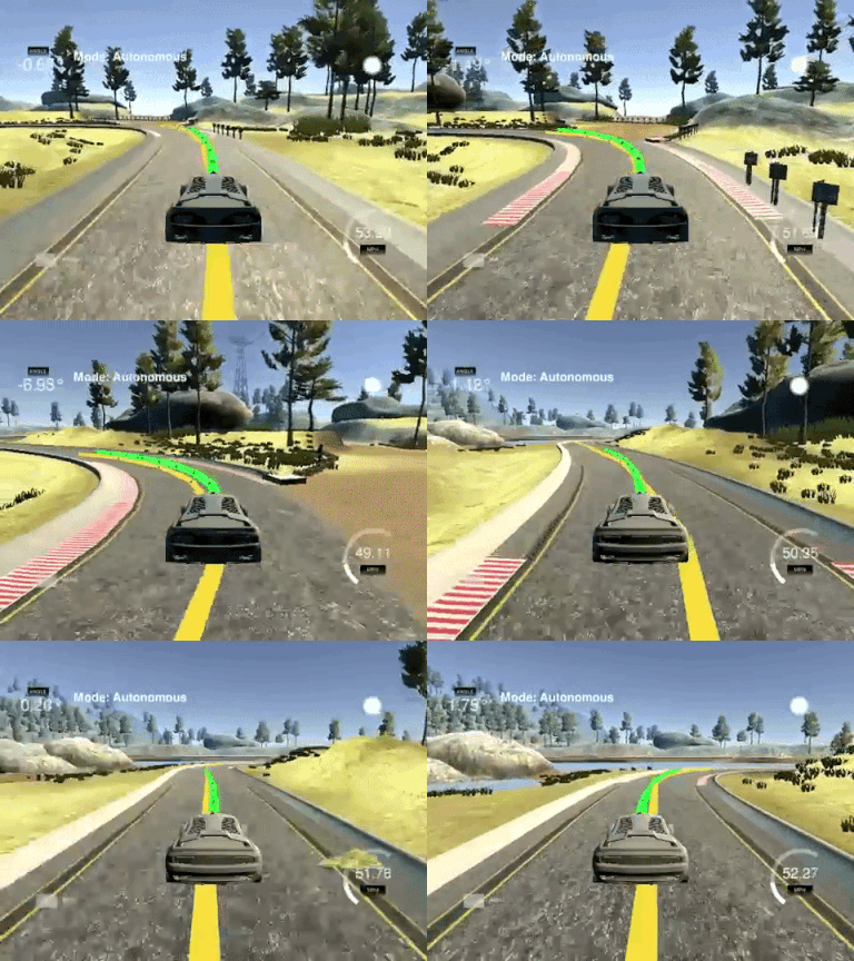
The goal of this project is to build a controller, using Model Predictive Control, that can safely drive an autonomous car around the track in Udacity's Self-Driving Car simulator.

Vehicle Model

The present MPC implementation is based on a kinematic vehicle model. These models are simplifications of dynamic models where tire forces, gravity, mass, and other real-world effects are ignored. Nevertheless, a kinematic model is justified in our case, since these models are more tractable and have a reasonable performance at low and moderate speeds.

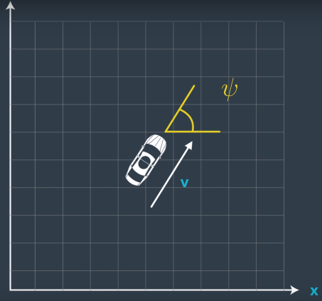
The state of the vehicle is given by its x and y position, heading psi, and velocity v, as represented in the following figure:

Actuator inputs allow us to control the vehicle state. Cars typically have three main actuators: steering wheel, acceleration pedal, and brake pedal. For simplicity, acceleration / brake pedals are considered a single actuator, with positive values for acceleration and negative values for braking. Hence, actuators are reduced to two control inputs: steering angle, delta, and acceleration a.

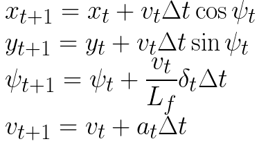
The state [x, y, psi, v] changes overtime based on the previous state and current actuator inputs [delta, a], as established by the following update equations:

Where L_f is related to the distance between the front of the vehicle and its center of gravity. The larger the vehicle, the slower the turn rate.

A controller actuates the vehicle to follow the reference trajectory within a set of design requirements. To quantify the deviation of the vehicle's actual and predicted paths with respect to the reference trajectory, two key metrics are monitored:

• Cross Track Error, cte: The distance between the reference trajectory and the vehicle's position. A naive first approximation to CTE can be cte = f(x) - y, where f is the reference trajectory fitted polynomial, and [x,y] the position of the car.
• Orientation Error, epsi: The difference between the actual orientation of the car, psi, and the desired orientation: epsi = psi - psi_des. At each point, the desired orientation is defined as the direction that is tangential to the reference trajectory, hence psi_des = atan(f'(x)), where f' is the derivative of the fitted polynomial f.

The errors can be monitored over time by integrating them into the state vector, and deriving the kinematic model around the new state vector [x, y, psi, v, cte, epsi]. The resulting update equations for the error components are:

The naive CTE definition becomes ill-defined in situations where the trajectory is parallel to the y-axis. Assuming moderate orientation error, this definition is noticeably more robust in the vehicle's local frame of reference, and can be further simplified since the state of the vehicle in its local coordinate system [x, y, psi] is constantly [0, 0, 0].

Since the error expressions become much simpler, the MPC optimization problem will be resolved in local coordinates.

At each instant, the reference trajectory waypoints given in map coordinates are transformed to the car's FoR via a 2D transformation where the rotation of the local system is equal to psi, and the origin is equal to the car's position [x, y]. The state vector in local FoR becomes [x, y, psi, v] = [0, 0, 0, v].

Cost function

The cost function has been defined to penalize:

• Cross track error
• Orientation error
• Large actuator inputs
• Rate of change of actuator inputs
• High velocities combined with sharp steerings

These error terms involve variables of heterogeneous nature: longitudinal and angular errors, steering and acceleration values, that are being blended into a unique metric. Weights must be applied to each term in order to equalize orders of magnitude.

In this project I have applied weights in the form of scaling parameters: each term is made non-dimensional and taken to the unity order of magnitude for design driving conditions, with the convenience that they can be physically reasoned, making tuning easier and more intuitive. For instance, the following code snippet illustrates how to heavily penalize deviations over 5 m/s with respect to the reference velocity:

double v_nd = 5;
fg[0] += CppAD::pow((vars[v_start + t] - ref_v) / v_nd, 2);

Latency

In a real car, actuation commands do not execute instantly, there is a delay as the command propagates throught the system. Realistic delays are in the order of 100 milliseconds.

This issue is known as latency, and it is an important challenge for certain controllers like PID, since it leads to instability if not appropiately accounted for.

The key fact is that given the current state and the resulting optimal actuation, due to latency the control command will not be effectivelly applied until a later state, that obviously does not correspond with the state the command was actually optimized for.

A way to overcome this is to set the initial state of the vehicle at a given instant not equal to the actual current state, but to a corrected state. This corrected state is the result of predicting the vehicle's state after a time step equal to latency, assuming the actuator inputs are constant and equal to the latest effectively applied values.

px += v * cos(psi) * dt_lat;
py += v * sin(psi) * dt_lat;
psi += - v * steer_value / Lf * dt_lat;
v += throttle_value * dt_lat;

where dt_lat is the latency time step, and steer_value and throttle_value are recovered from the car's telemetry.

In summary, the corrected state defined above would constitute the actual current state for all the subsequent operations:

• Transformation of waypoints and car position from global to local frame of reference.
• 3rd order polynomial fitting to reference trajectory
• Actuator optimization

This correction can be disabled via the lat_predict flag in main.cpp.

Timestep lenght and elapsed duration

Driving the car at moderate speeds (say 50 mph) using a 2-second horizon involves optimizing the upcoming 40-50 meters. These figures are reasonable given the morphology of the simulator circuit.

Hence, we are considering N * dt near to 2. Starting with dt = latency, the vehicle is unstable: the car is hardly able to keep track in a straight line since it constantly overshoots its control corrections. Behaviour becomes worse when dt is decreased. Acceptable performance was achieved with dt > latency, in particular choosing time steps around 0.2. In this YouTube link you can find a video of a successfull run using N = 10 and dt = 1.8.

Dependencies

• cmake >= 3.5
• All OSes: click here for installation instructions
• make >= 4.1(mac, linux), 3.81(Windows)
  • Linux: make is installed by default on most Linux distros
  • Mac: install Xcode command line tools to get make
  • Windows: Click here for installation instructions
• gcc/g++ >= 5.4
  • Linux: gcc / g++ is installed by default on most Linux distros
  • Mac: same as make - [install Xcode command line tools]((https://developer.apple.com/xcode/features/)
• uWebSockets
  • Run either install-mac.sh or install-ubuntu.sh.
  • If installed from source, checkout to commit e94b6e1, i.e.

    git clone https://github.com/uWebSockets/uWebSockets 
    cd uWebSockets
    git checkout e94b6e1
    

    Some function signatures have changed in v0.14.x. See this PR for more details.
• Fortran Compiler
  • Mac: brew install gcc (might not be required)
  • Linux: sudo apt-get install gfortran. Additionally gcc and g++ should be installed, sudo apt-get install gcc g++. Look in this Dockerfile for more info.
• Ipopt
  • Mac: brew install ipopt
    • Some Mac users have experienced the following error:

    Listening to port 4567
    Connected!!!
    mpc(4561,0x7ffff1eed3c0) malloc: *** error for object 0x7f911e007600: incorrect checksum for freed object
    - object was probably modified after being freed.
    *** set a breakpoint in malloc_error_break to debug
    

    This error has been resolved by updrading ipopt with brew upgrade ipopt --with-openblas per this forum post.
  • Linux
    • A version of Ipopt 3.12.1 or higher is needed. The version available through apt-get is 3.11.x. In any case, this repo provides a script install_ipopt.sh that will install Ipopt. You just need to download the source from the Ipopt releases page.
    • Then call install_ipopt.sh with the source directory as the first argument, ex: sudo bash install_ipopt.sh Ipopt-3.12.1.
• CppAD
  • Mac: brew install cppad
  • Linux sudo apt-get install cppad or equivalent.
• Eigen. This is already part of the repo so you shouldn't have to worry about it.
• Simulator. You can download these from the releases tab.
• Not a dependency but read the DATA.md for a description of the data sent back from the simulator.

Basic Build Instructions

1. Clone this repo.
2. Make a build directory: mkdir build && cd build
3. Compile: cmake .. && make
4. Run it: ./mpc.

Code Style

In this project, I have stuck to Google's C++ style guide.