CarND: Vehicle Detection and Tracking 
The goal of this project is to build a software pipeline to detect and track surrounding vehicles in a video stream generated by a front-facing camera mounted on a car.
At its core, this pipeline uses a machine learning model to classify video frame patches as vehicle or non-vehicle.
The project is separated into two well-differentiated blocks:
- Training stage: feature extraction pipeline for the training dataset, and model training.
- Prediction stage: feature extraction pipeline for the video stream frames.
It is possible to create a unique feature extraction pipeline that suits both training and prediction stages. However, this is not optimal since it would require a computationally expensive sliding window search implementation to predict on the new input video frames. This will be discussed later in more detail.
Project structure
The project workflow is built in the notebook p5_solution.ipynb, linked here. To improve the readability of the notebook and make it less bulkier, the basic core methods and other helpers have been extracted to the aux_fun.py script. These functions are cited here as aux_fun.method_name(), whereas those that are defined in the actual project notebook are simply cited as method_name().
Training set construction
To train the classifier, a combination of the GTI vehicle image database and the KITTI vision benchmark suite has been used. The merged database contains labelled 64 x 64 RGB images of vehicles and non-vehicles, in a near-50% proportion.
| Positive | Negative | Total |
|---|---|---|
| 8792 | 8968 | 17760 |
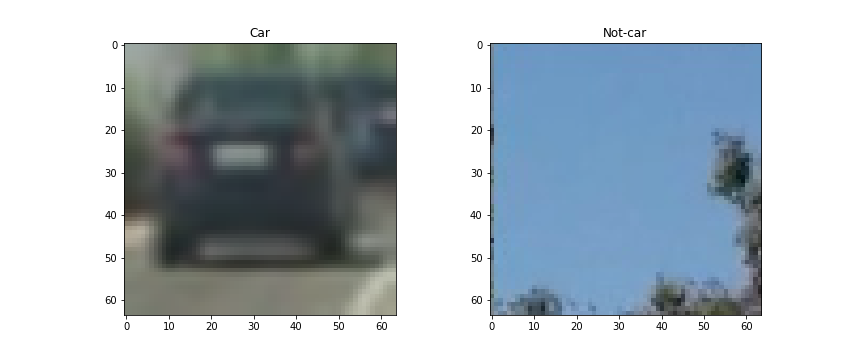
Here is an example of each class:
Three types of features are extracted from the images in this project:
- Histogram of Oriented Gradients (HOG), using
aux_fun.extract_hog_features(). - Color histogram features, using
aux_fun.extract_hist_features(). - Spatial features, i.e. resized image raw pixel values, using
aux_fun.extract_spatial_features().
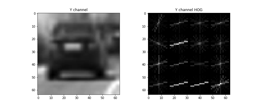
For the initial car example, the HOG features extracted from the Y channel using 9 orientation bins, 16 pixels per cell, and 2 cell per block:
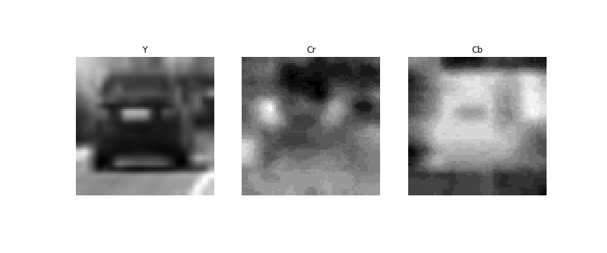
The pixel values in YCrCb space:
And finally the 32-bin histograms for each of the YCrCb channels:
To be consumable by the classifier model, the feature arrays must be flattened and concatenated together into a one-dimensional vector.
For a single image, the resulting feature vector extraction is encapsulated in aux_fun.extract_single_img_features(). This processed is looped for each image in the database with the help of aux_fun.extract_features_from_img_file_list(). Finally aux_fun.build_dataset() merges and shuffles all the data into the final training set, and provides the label vector populated with zeros and ones.
Model training pipeline
The model used for the classication task is a Linear Support Vector Machine Classifier, in particular sklearn.svm.LinearSVC. This election is supported on the fact it is a method that is known to perform well in image classification taks, while being faster than higher order kernel SVMs and complex tree based models. It is important for the model to be fast at predicting, since it must be able to be part of a video stream.
The training set construction involved the joint usage of features that present disparity of magnitudes: gradient values, raw pixel values, and histogram counts. It is therefore necessary to perform a scaling of the features so one type does not dominate over the rest during the training process.
Feature scaling is performed using sklearn.preprocessing.StandardScaler. A great advantage of using scikit-learn's API, is that preprocessing steps can be enclosed together with the model itself in a pipeline object, sklearn.pipeline.Pipeline, that exposes the same methods than the classifier, but without having to worry about explicitly calling the preprocessing steps everytime the model is used, improving readability and robustness.
The pipeline object is built with the sklearn.pipeline.make_pipeline() method:
from sklearn.pipeline import make_pipeline
from sklearn.preprocessing import StandardScaler
from sklearn.svm import LinearSVC

scaled_clf = make_pipeline(
    StandardScaler(),
    LinearSVC()
)
The effect of the hyperparameters on the performance of the model is assessed using a 3-fold stratified cross validation, to ensure the 50-50 class balance is preserved in each fold.
Combined assessment using CV (over 99% accuracy with low variance) and the test images leaded to the usage of the following parameters:
PARAMS = {
    'use_spatial': True,
    'spatial_cspace': 'YCrCb',
    'spatial_resize': 32,

    'use_hist': True,
    'hist_cspace': 'YCrCb',
    'hist_nbins': 32,

    'use_hog': True,
    'hog_cspace': 'YCrCb',
    'channels_for_hog': [0,1,2],
    'hog_orientations': 9,
    'hog_pixels_per_cell': 16,
    'hog_cells_per_block': 2,

    'cells_per_step_overlap': 1
}
Also, C=10 for the regularization parameter of the SVM proved to have a good performance.
In summary, the YCrCb color space is used in all the stages of feature extraction: HOG applied to all channels, YCrCb 32-bin histograms, and YCrCb color information. YCrCb turned out to be a lot more robust than RGB agains variations in lighting conditions.
NOTE: The GTI image database contains multiple images for each real world entity, since the images have been extracted from near-to-consecutive video frames. If this fact is not taken into account, the obtained CV scores will be overly optimistic due to leakage: it is possible to find images corresponding to the same entity in both training and validation folds at each step. This could be easily resolved using time series data or entity-labelled data together with a Group K-Fold method, sklearn.model_selection.GroupKFold.
This extra information is not available. I tried defining clusters based on template matching with cv2.matchTemplate(), where images with high resemblance would be grouped together, but was not robust enough. Further approaches were not tried due to lack of time.
Prediction pipeline
The peculiarity of the prediction stage is that the inputs are video frames, that must be hovered by a sliding window that extracts features for the model to decide if the window's region is a vehicle or not.
The objective is to perform a sliding window search, with a given value of overlap in both directions of space, and extract all the features (recall HOG, color histograms, and spatial features) for each window providing a prediction. However, this approach is overly computationally expensive, since features are extracted multiple times in a given region due to window overlapping.
A more efficient solution is to extract the HOG features only once, on the whole image, and subsample the resulting array along with the moving windows. This improved methodology is encapsulated in aux_fun.find_cars().
In this implementation, window scale is controlled with the scale parameter. The scale parameter resizes the image so that the sliding windows have an effective size of 64*scale.
Overlapping is controlled with the relation between the total number of HOG cells in a 64-px window and cells_per_step_overlap. An example: regardless of the scale, hog_pixels_per_cell=16 involves 4 x 4 cells in a 64 x 64 window. Hence, cells_per_step_overlap=1 yields 75 % overlap, cells_per_step_overlap=2 50 %, and so on.
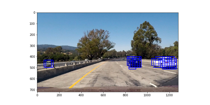
The following image shows the detections with scale 1.0 windows and 75 % overlap:
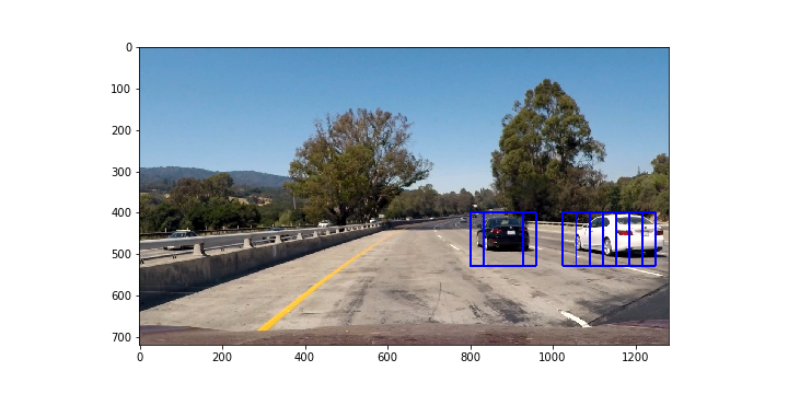
whereas the image bellow presents detections with a 2.0 scale (128 x 128 windows) and 75 % overlapping:
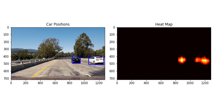
As seen, in a given frame there are many overlapping positive detections surrounding the vehicles, but there can also be false positives. False positives tend to appear in a sparse manner, so their presence in a frame can be resolved by building tight bounding boxes to the hot regions in a thresholded heatmap. Continuing with the example case from above:
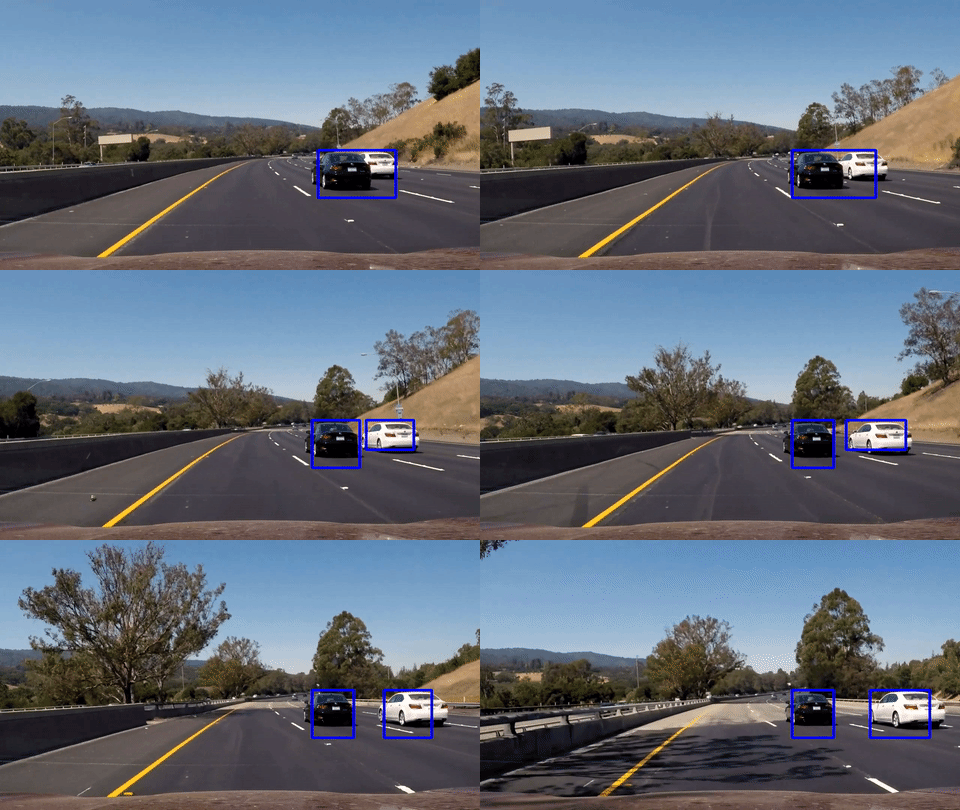
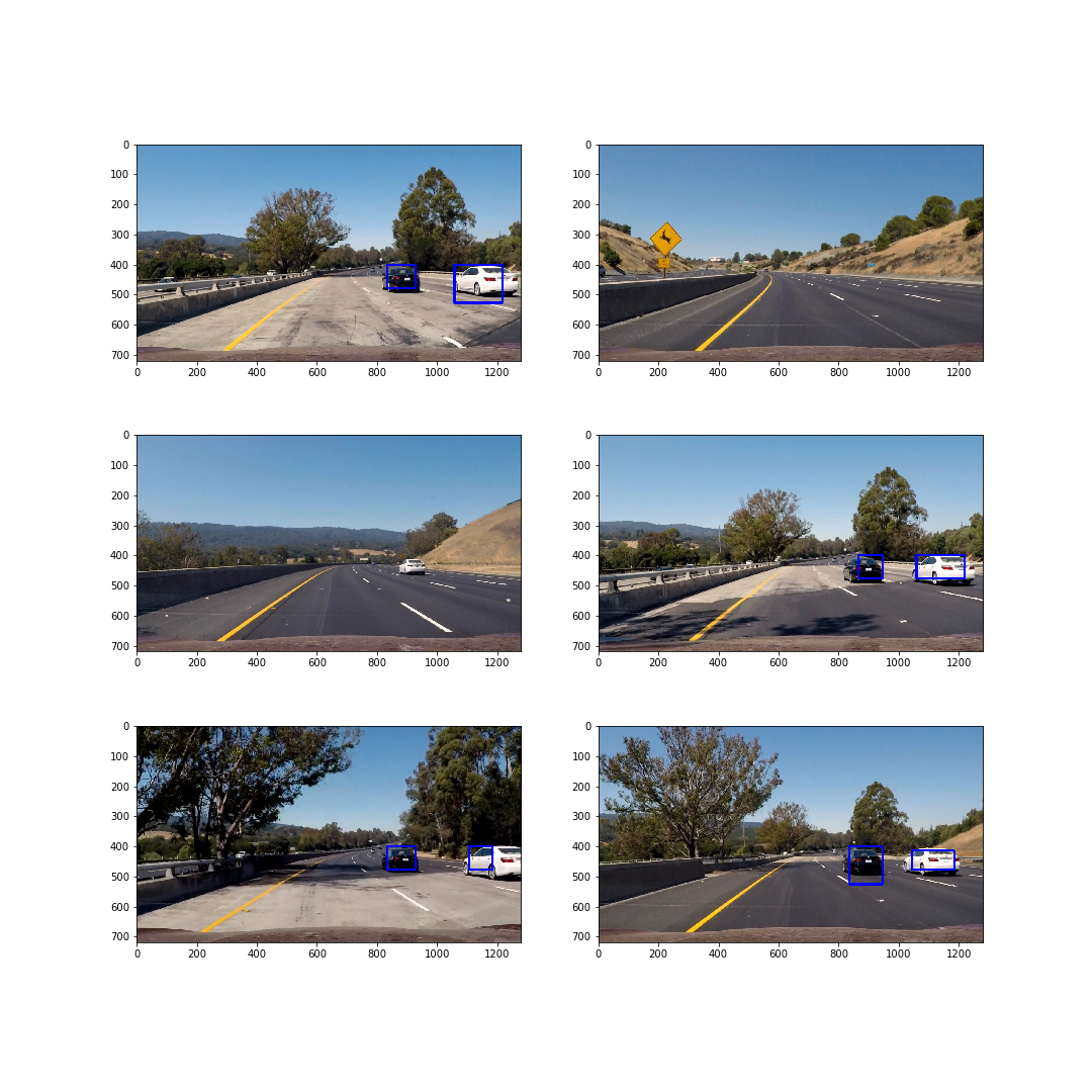
This methodology is encapsulated in static_image_pipeline(). This method applied to different test images produces:
Video implementation
At this point static_image_pipeline() can process video inputs. Although it manages to track vehicles correctly, the bounding box is flickering, and in some frames, the pipeline is not able to detect cars, and the tracking is interrupted during fractions of seconds.
To solve this, and further mitigate the appearance of false positives, the heatmaps generated at each frame are recursively weight-averaged with the previous ones and thresholded, to eventually apply tight bounding boxes to the high-confidence areas.
This is accoumplished with the VehicleTracker class and its process_frame() method, which is directly fed to the clip generator once instantiated.
In the final pipeline, window search is applied on 3 different scales (scale = 1.0, 2.0, 3.0), having taken into account that cars are smaller the nearer they are to the horizon of the image, with a overlap of 75 %.
This setup performed very well, only finding false positives in very few frames, that correspond to cars circulating in the opposite direction, so technically they could be treated as true positives.
The solution video is included in the repo, named project_video_solution.mp4. You can also find here a YouTube link to the video.
Challenge
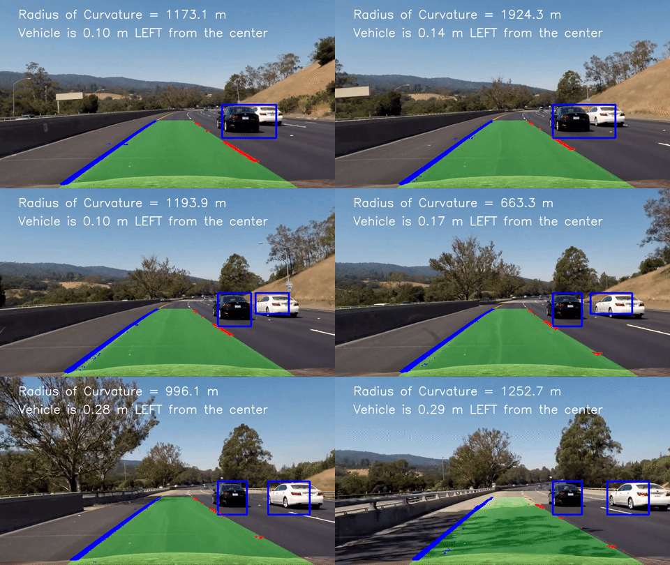
The vehicle detection pipeline has been combined with the lane detection pipeline in the notebook p5_challenge_solution.ipynb, linked here.
In this new approach the VehicleTracker class has been extended to keep track of the lanes trough the Line class and the lane_detection_pl() method. The core methods for lane detection can be found in the p4_aux.py script, while the camara distortion parameters, and source/destination points definition are saved as pickles in the challenge folder.
The solution video is located in the latter folder, and named as challenge_solution.mp4. A YouTube link is also provided.

