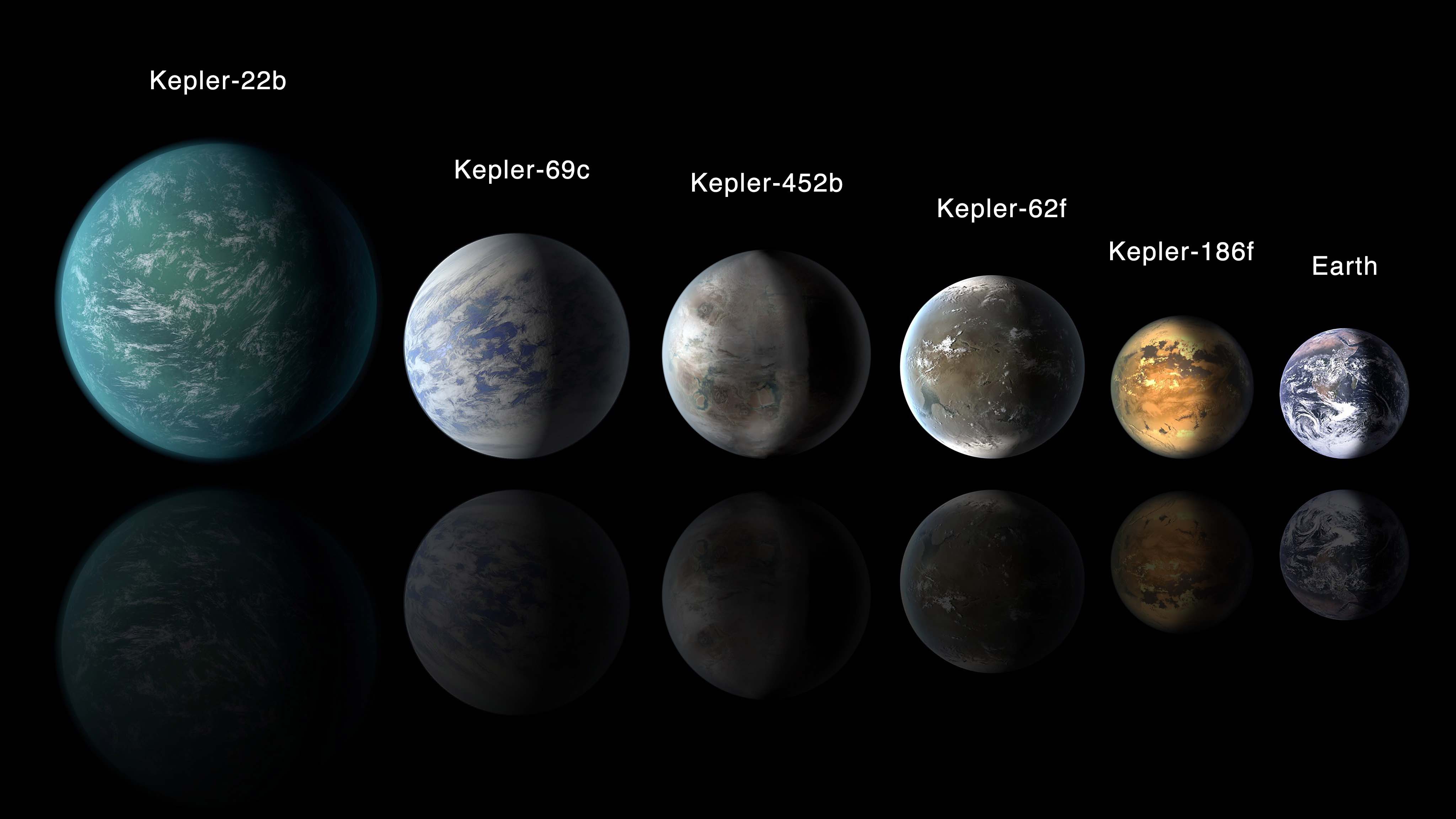
This exercise was based on data collected on potential planets outside of our solar system ("exoplanets"). Over a period of nine years in deep space, the NASA Kepler space telescope conducted a planet-hunting mission to discover hidden planets outside of our solar system. The resulting dataset includes data on objects considered potential candidates for exoplanet classification, with information on various features that could be used to determine it's candidacy as an exoplanet, as well as the final classification. The purpose of this exercise was to create machine learning models capable of classifying candidate exoplanets from the raw dataset by evaluating data collected during this period.
Data Source: https://www.kaggle.com/nasa/kepler-exoplanet-search-results
Further information on the Keplar data, including a glossary of the individual features, is available at: https://exoplanetarchive.ipac.caltech.edu/docs/API_kepcandidate_columns.html#pdisposition
Steps for creating the models:
- Preprocessing the raw data
- Tuning the models
- Comparing the models
- Preprocessing the dataset prior to fitting the model.
- Performing feature selection and remove unnecessary features.
- Using
MinMaxScaler(initially) to scale the numerical data. - Separating the data into training and testing data.
- Useing
GridSearchto tune model parameters. - Tuning and comparing at least two different classifiers.
Model 1 SVM
After reading in the data, I had to decide which features to keep for the model. For the initial model, I decided to eliminate err1 and err2 columns for all features, and keep just the initial data column for each feature (period, time, impact, duration, depth, etc). After that, I assigned x and y values for the model, and then split the data into "train" and "test" subsets. The data were then scaled and normalized to improve accuracy, with smaller gaps between data points (i.e. adjusting the weighting of each point) within the model. Lastly, GridSearchCV was used to tune the model's parameters.
Initial results Training Data Score: 0.8167079916078581 Testing Data Score: 0.7946224256292906
GridSearchCV tuning 0.82052260156399
The GridSearchCV tuning did improve the accuracy of the model a bit, but the model seemed to have some space for improvement.
Model 2 Logistic Regression
The data cleaning and preprocessing steps were the same as for model 1. In this model, StandardScaler was used to scale and onrmalize the data instead of MinMaxScaler, with slightly better results.
Training Data Score: 0.8247186725157353 Testing Data Score: 0.8089244851258581
The results after using GridSearchCV to tune the model's parameters show more noticable improvement: 0.8331108144192256
Model 3 All Data Fields
The final model included all of the data from the data set, without eliminating any of the columns, essentially restoring the err1 and err2 columns. This noticeably improved the accuracy of the model.
Training Data Score: 0.8922372687392714 Testing Data Score: 0.8884439359267735
Results after using GridSearchCV to tune the model's parameters only showed slight improvements 0.8891855807743658
Model 3 produced the best results, with the performance after tuning with GridSearchCV being the best, but not significantly better than the initial model. For all three models, changing the grid parameters for C and gamma values did not produce any score improvement.
