A Python library for visualizing a Sumo network and trajectories with matplotlib or as an OBJ file.
Network and Trajectory Plotting
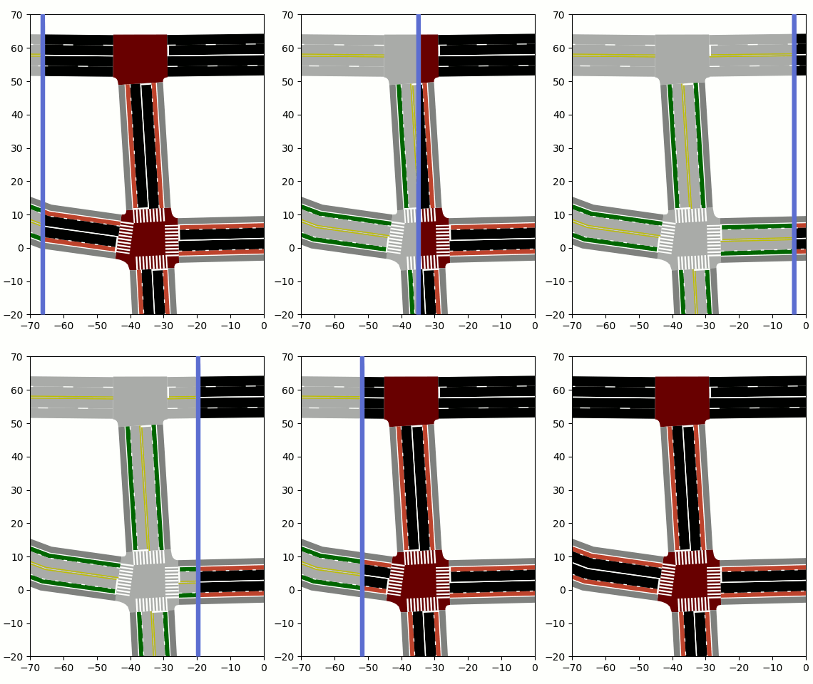
Highly Customizable
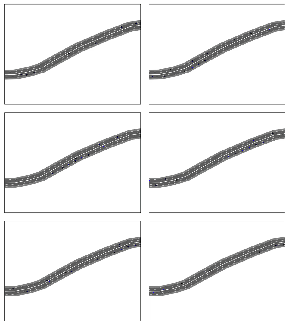
Trajectory Animation
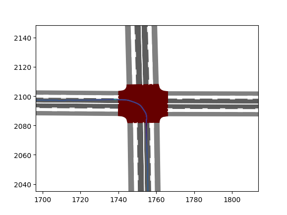
Basic trajectory plotting from FCD outputs is built in, but it is also possible to plot custom data and graphics on top of the network with the full flexibility and power of matplotlib and other compatible libraries, such as seaborn.
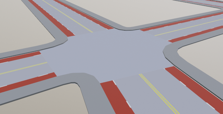
3D geometry for a network can be generated and saved as a Wavefront-OBJ file.

This package can be installed via pip with the command pip install SumoNetVis.
You can then import the library with:
import SumoNetVis- shapely (>=1.7.0 for stop lines and OBJ export)
- triangle (for OBJ terrain export)
- matplotlib
- numpy
To plot a Sumo net file and trajectories, you can use the following code:
import SumoNetVis
import matplotlib.pyplot as plt
# Plot Sumo Network
net = SumoNetVis.Net("path/to/yourfile.net.xml")
net.plot()
# Plot trajectories
trajectories = SumoNetVis.Trajectories("path/to/fcd-output.xml")
trajectories["vehicle_id"].assign_colors_speed()
trajectories["vehicle_id"].plot()
# Show figure
plt.show()
the Net.plot() function takes the following optional parameters:
- ax: matplotlib Axes object (defaults to currently active Axes)
- clip_to_limits: if True, only objects visible in the current view extents will be drawn
- zoom_to_extents: auto-zoom to Net extents (defaults to True)
- style: lane marking style to use ("USA" or "EUR")
- stripe_width_scale: scale factor for lane marking widths (defaults to 1)
- plot_stop_lines: whether to plot stop lines
- apply_netOffset: whether to translate the network by the inverse of the netOffset value
- lane_kwargs: dict of kwargs to pass to the lane plotting function (matplotlib.patches.Polygon()), for example alpha
- lane_marking_kwargs: dict of kwargs to pass to the lane markings plotting function (matplotlib.lines.Line2D())
- junction_kwargs: dict of kwargs to pass to the junction plotting function (matplotlib.patches.Polygon())
Any kwargs passed directly to Net.plot() will be passed to each of the plotting functions. These will, however,
be overridden by any object-type-specific kwargs (lane_kwargs, etc.).
To plot all junctions at 50% opacity and all other objects at 80% opacity, for example, one can use:
net.plot(junction_kwargs={"alpha": 0.5}, alpha=0.8)The color scheme of junctions and various lane types can be customized by modifying entries in the global variable
COLOR_SCHEME. For example, to plot bike lanes as dark green instead of dark red, do the following:
SumoNetVis.COLOR_SCHEME["bicycle"] = "#006600"Any color specification supported by matplotlib can be given here, such as RGB and RGBA hex strings and float tuples, as well as color names and abbreviations. See the matplotlib documentation for more detailed information.
When using the various "assign_colors" functions, when applicable, a corresponding matplotlib ScalarMappable will
be stored in the Trajectory.mappable property. The Trajectories class also contains a property,
mappables, which contains a dict of vehID: ScalarMappable pairs. Therefore, to automatically generate a
colorbar, one of the two following (equivalent) methods can be used:
plt.colorbar(trajectories["vehicle_id"].mappable)
# OR
plt.colorbar(trajectories.mappables["vehicle_id"])Instead of visualizing Trajectories as lines, an animation can be generated using the matplotlib.animation module.
import matplotlib.animation as animation
trajectories = SumoNetVis.Trajectories("path/to/fcd-output.xml")
fig, ax = plt.subplots()
a = animation.FuncAnimation(fig, trajectories.plot_points, frames=trajectories.timestep_range(), repeat=False,
                            interval=1000*trajectories.timestep, fargs=(ax,), blit=True)
plt.show()
The plot settings for each vehicle can be customized and the color of each point can be animated, as shown in the following example.
for trajectory in trajectories:
        trajectory.assign_colors_speed()
        trajectory.point_plot_kwargs["ms"] = 8  # set marker size. Can set any kwargs taken by matplotlib.pyplot.plot().
In order to animate the color of the points based on the assigned color scheme, an additional farg must be passed when creating the animation.
a = animation.FuncAnimation(fig, trajectories.plot_points, frames=trajectories.timestep_range(), repeat=False,
interval=1000*trajectories.timestep, fargs=(ax, True), blit=True)Currently, polygons, POIs, and bus stops are supported. Sumo additional files can be loaded and plotted in one of two ways:
Load directly with Network
net = SumoNetVis.Net("path/to/yourfile.net.xml", additional_files="path/to/additionals_file.add.xml")Load and handle additional files separately
addls = SumoNetVis.Additionals("path/to/additionals_file.add.xml", reference_net=net)
addls.plot()
The reference_net argument is optional, and only necessary for bus stops and for POIs whose position is defined
relative to a lane in the network.
Several styles of bus stop are supported. The style can be changed using the function
SumoNetVis.set_bus_stop_style(). See documentation for further details
Generic parameter values are loaded for supported objects (edges, lanes, junctions, vehicles, polys) and are stored in
an attribute called params in each of the respective object classes. These can be used to aid in implementing
custom functionality on top of SumoNetVis. There are also some built-in features which can make use of these parameters.
For example:
- trajectory colorization
- OBJ export material
- OBJ export extrude height
See the Sumo documentation on generic parameters as well as the full SumoNetVis documentation for more information.
The Wavefront-OBJ format is a text-based file format. The Net.generate_obj_text() method generates the contents
of this file for the given Sumo network. In order to save an OBJ file, do the following:
# Save a network as an OBJ file
with open("model.obj", "w") as f:
    f.write(net.generate_obj_text())

# Save bus stops and polygons from an additional file as an OBJ file
with open("busstops.obj", "w") as f:
    f.write(addls.generate_bus_stops_obj_text())
The axis configuration in the generated file is Y-Forward, Z-Up. Check these settings if the orientation of the model is incorrect when importing the file into a 3D modelling program.
A flat planar "terrain" mesh can optionally be generated for all areas within a given distance of a network object. See full documentation for further information.
Each type of object is defined with a corresponding material (i.e. all bike lanes have the same material, all sidewalks, and so on), making it easy to quickly set the desired material properties before rendering. These can also be mapped to user-defined material names if desired (see full documentation). Default material names are of the following forms: for markings, "[c]_marking", where [c] is the marking color ("w" for white, "y" for yellow, etc.); for lanes, "[type]_lane", where [type] is the lane type ("pedestrian", "bicycle", "no_passenger", "none", "other"); for junctions, "junction"; for terrain, "terrain".
To aid in extensibility, each plotting function returns an iterable object consisting of all matplotlib Artist objects
generated by that function. Trajectory plotting functions return simple lists or tuples. Net and Additionals plotting
functions return an ArtistCollection object which is iterable just like a normal list, but also contains a list
attribute for each object type. Each artist is also given an attribute sumo_object which contains a reference to
the SumoNetVis object that generated it. The artists can then be acted on as desired, for example to create custom
animations or to make an interactive plot. An illustrative example of the latter is shown below. In the example,
when a user clicks on a lane, that lane's id and speed properties are printed out.
def onpick(event):
    sumo_object = event.artist.sumo_object
    print("Lane ", sumo_object.id, "clicked. Speed limit: ", sumo_object.speed)

artists = net.plot()
for lane_artist in artists.lanes:
    lane_artist.set_picker(True)
fig.canvas.mpl_connect("pick_event", onpick)
plt.show()API documentation can be found here
Issues and pull requests are welcome.


