The program reads in an ascii data file with two columns:
- col 1 = variable (e.g hand position along left-right axis)
- col 2 = binary response (0,1) (e.g. "left" vs "right" sensed hand position)
and fits a binomial model + logit link function using maximum likelihood estimation. A good tutorial on MLE is:
The model is of the form:
y = b0 + (b1 * x)
p(x) = Pr(response|x) = 1 / (1 + exp(-y))
The model parameters b0 and b1 are found that minimize the negative log-likelihood of the data. This is done using numerical optimization. The Nelder-Mead simplex algorithm is used here. The code makes use of Michael Hutt's implementation of the Nelder-Mead algorithm.
The program outputs to the screen:
- the model parameters b0 and b1,
- the bias (the x value at the 50th percentile) and
- the slope at the 50th percentile
- the acuity (the distance in x between the 25th and 75th percentile)
The program also generates three output files:
- _params
- b0, b1, bias, slope, x75, x25, x72-x25
- _pred: p(x) for 50 x points across the range of input x
- _dist: model param distribution based on parametric bootstrap
an example data file is exdata
gcc -Wall -o psychometric psychometric.c nmsimplex.c
./psychometric exdata 10000
found 154 rows of data in exdata
***************************************************************
y = 0.60417 + (0.48711 * x)
p(r|x) = 1 / (1 + exp(-y))
***************************************************************
bias = -1.24031
slope at 50% = 0.12178
acuity (x75 - x25) = (1.01504 - -3.49566) = 4.51070
***************************************************************
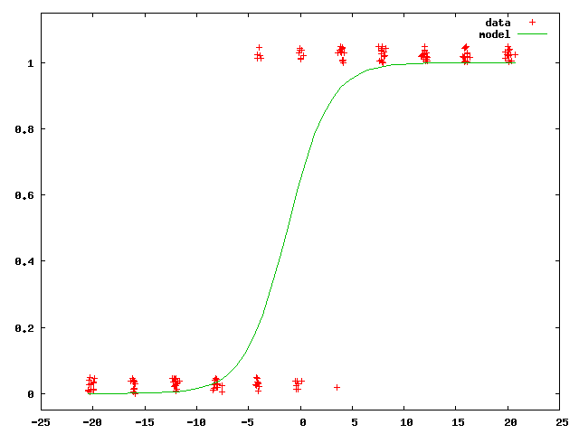
gnuplot commands to plot result:
set yrange [-.05:1.15]
plot 'exdata' using 1:($2 + (rand(0)/20)) title 'data' with points, \
     'exdata_pred' using 1:2 title 'model' with lines
***************************************************************
parametric bootstrap: simulating 10000 times...
done
An example of the graphic produced by the gnuplot commands for exdata is shown below. Note that the data are offset in y using random values, to help with visualization of the (binary) responses.
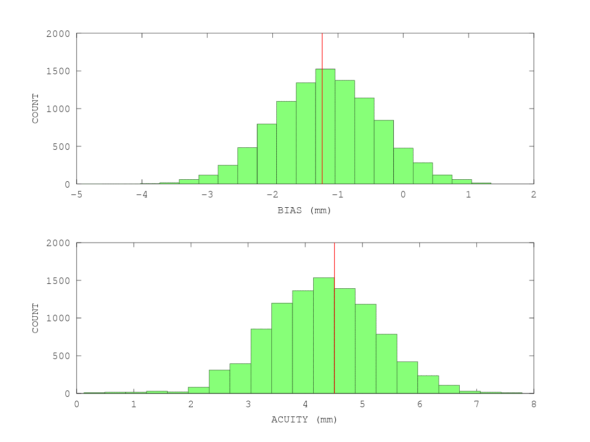
You can have a look at the bootstrap distributions of the parameters like so: here I use GNU Octave:
load exdata_dist
figure
subplot(2,1,1)
hist(exdata_dist(:,3),21)
xlabel('BIAS (mm)')
ylabel('COUNT')
load exdata_params
line([exdata_params(3) exdata_params(3)],get(gca,'ylim'),'color','r','linewidth',2)
subplot(2,1,2)
hist(exdata_dist(:,7),21)
xlabel('ACUITY (mm)')
ylabel('COUNT')
line([exdata_params(7) exdata_params(7)],get(gca,'ylim'),'color','r','linewidth',2)
print exdata_dist.png -dpng

