The goals / steps of this project are the following:
- Compute the camera calibration matrix and distortion coefficients given a set of chessboard images.
- Apply a distortion correction to raw images.
- Use color transforms, gradients, etc., to create a thresholded binary image.
- Apply a perspective transform to rectify binary image ("birds-eye view").
- Detect lane pixels and fit to find the lane boundary.
- Determine the curvature of the lane and vehicle position with respect to center.
- Warp the detected lane boundaries back onto the original image.
- Output visual display of the lane boundaries and numerical estimation of lane curvature and vehicle position.
My project includes the following files:
README.mdwriteup summarizing the resultslane.pycontaining the code for creating the lane detection videocv.pya collection of computer vision utilities functionsAdvanced_Lane_Lines.ipynba jupyter notebook with step by step details of the lane detection pipelineproject_video_output.mp4containing the lane detection results
The code for this step is contained in lines 8 through 45 of the file called cv.py:
I start by preparing "object points", which will be the (x, y, z) coordinates of the chessboard corners in the world.
Here I am assuming the chessboard is fixed on the (x, y) plane at z=0, such that the object points are the same for
each calibration image. Thus, objp is just a replicated array of coordinates, and objpoints will be appended with a
copy of it every time I successfully detect all chessboard corners in a test image. imgpoints will be appended with
the (x, y) pixel position of each of the corners in the image plane with each successful chessboard detection.
I then used the output objpoints and imgpoints to compute the camera calibration and distortion coefficients
using the cv2.calibrateCamera() function. I applied this distortion correction to the test image using the
cv2.undistort() function and obtained this result:
To demonstrate this step, the code below shows how I apply the distortion correction:
img = cv2.imread('test_images/straight_lines1.jpg')
img = cv2.cvtColor(img, cv2.COLOR_BGR2RGB)
objpoints, imgpoints = load_calibration_parameters(6, 9)
img_undistort = undistort(img, objpoints, imgpoints)
I experimented with different several color thresholding and gradient techniques, as shown in the image below:
I ended using a combination of color and gradient thresholds to generate a binary image (steps at
lines 126 through 153 in cv.py). Here's an example of my output for this step:
The above binary image is the result of applying the or operation over the following color thresholds an gradients
transformations:
The code for my perspective transform includes a function called warper(), which appears in lines 195 through 200
in the file cv.py. The warper() function takes as inputs an image (img), as well as source (src) and destination (dst) points.
I chose the hardcode the source and destination points in the following manner:
height, width = img.shape[0], img.shape[1]
src = [
    ((width // 2) - 70, (height // 2) + 110),
    ((width // 2) + 80, (height // 2) + 110),
    (width - 170, height),
    (0 + 220, height)
]
dst = [
    (width // 4, 0),
    (width - width // 4 - 40, 0),
    (width - width // 4 - 40, height),
    (width // 4, height)
]
This resulted in the following source and destination points:
| Source | Destination |
|---|---|
| 570, 470 | 320, 0 |
| 720, 470 | 920, 0 |
| 1110, 720 | 920, 720 |
| 220, 720 | 320, 720 |
I verified that my perspective transform was working as expected by drawing the src and dst
points onto a test image and its warped counterpart to verify that the lines appear parallel
in the warped image.
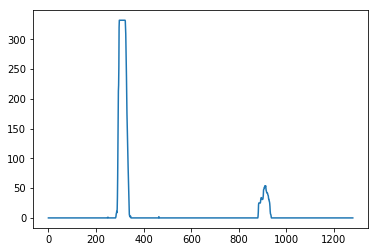
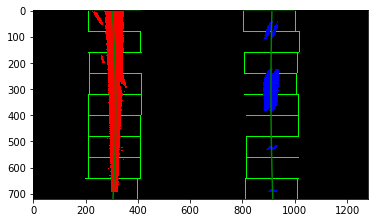
Then I used a histogram on the x-axis to fit my lane lines with a 2nd order polynomial kinda like this:
For each lane mark we fit a parabola with coefficients A, B and C as follow:
Our equation for curvature becomes:
Note that we need to multiple the pixel coefficients with a meter multiplier, to have the results in meters.
I implemented the curvature measurements in lines 170 through 178 in my code in lane.py
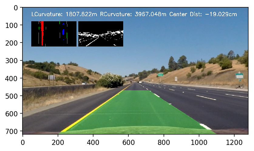
Finally, I used the function unwrap to project the lane back to the road, I implemented
this step in lines 180 through 205 in my code in lane.py. Here is an example of
my result on a test image:
Here's a link to my video result
Here I'll talk about the approach I took, what techniques I used, what worked and why, where the pipeline might fail and how I might improve it if I were going to pursue this project further.
My approach used the following techniques:
-
Combination of gradient (sobel-x) and color thresholds for yellow and white lane marks, this was really helpful since the multiple layers of threshold and gradient redundancy improve the quality of the binary image, thus improving lane detection. For instance, under low lighting conditions the RGB red threshold did not perform well, but the HSV yellow threshold worked quite good.
-
Smoothing by averaging the coefficients of the lane marks parabolas within the last 5 frames, this help avoiding bad frames from skew the detection results.
-
Filter out outlier frames by using a curvature threshold, same as the point above, improve lane detection for noisy frames.
If were to pursue this project further I will try to improve the following:
-
Consider different environment conditions, for instance, night, snow, etc. This can be improved by dynamic color thresholds.
-
Dynamic image wrapping points, at the moment the points are hardcoded, this will fail under lanes with a different configuration, consider for instance, wider or narrow lanes. A better approach will attempt to detect those control points.
-
Consider lanes with high curvature, in those cases just a section of the lane is visible, because of this drawing the lane should only depend upon one of the lane marks.
-
Consider not visible lanes, this could happen either for missing lane marks on the road or occlusion from other objects, in those cases we need to either extrapolate the lane based on the width of the road, or based on a estimation of previous measurements, my approach will fall apart on those cases.
-
Consider machine learning approach, it's possible to build a CNN to predict 4 points corresponding to the lane area.


