The goals / steps of this project are the following:
- Load the data set (see below for links to the project data set)
- Explore, summarize and visualize the data set
- Design, train and test a model architecture
- Use the model to make predictions on new images
- Analyze the softmax probabilities of the new images
- Summarize the results with a written report
I used numpy to calculate summary statistics of the traffic signs data set:
- The size of training set is 34,799
- The size of the validation set is 4,410
- The size of test set is 12,630
- The shape of a traffic sign image is 32x32x3, 32x32 pixels with 3 color channels (RGB).
- The number of unique classes/labels in the data set is 43
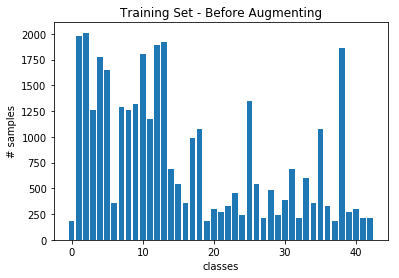
Here is an exploratory visualization of the data set. It is a bar chart showing how the traffic sign classes are distributed:
As a first step, I decided to convert the images to grayscale because noticed the shape of the image was a more important feature for the classification than the color.
As a second step, I normalized the image data because this will prevent the model for overfitting, since big values can lead to numerical error.
As a last step, I applied histogram equalization, which improves the contrast and brightness of the image, thus improving the classification task.
I decided to generate additional data because as can be seen from the histogram above, the data is not well distributed, some classes have many training examples, while others have just a few. For instance, class 0 (speed limit 20 km/h) have less than 250 training examples, while class 1 (speed limit 30 km/h) have almost 2,000.
To add more data to the the data set, I used the following techniques rotations, vertical and horizontal flips and random noise because of the following reasons:
-
Rotations: This will allow the classifier to learn rotations invariance, and be more robust.
-
Vertical and Horizontal Flips: As can be seen in the training dataset, some traffic signs are not affected by horizontal flips, others are not affected by vertical flips, few of them are not affected by both kind of flips. Taking this into consideration, I used vertical and horizontal flips to generate more data, thus improving the classifier training set.
-
Random Noise: This kind of perturbation can help the classifier to be more robust, while facing noisy data.
Below a few examples of all the transformations applied to the traffic signs:
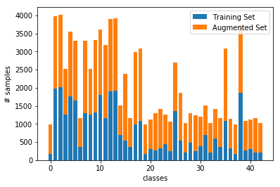
The difference between the original data set and the augmented data set is the following:
As you can see the augmented training improves the representation of each class in the dataset. All the classes are now over the mean of the training set, which was around 800 training samples.
The size for the augmented training set is 54460, additional 19661 were added to the original training set.
My final model consisted of the following layers:
| Layer | Description |
|---|---|
| Input | 32x32x1 Grayscale image |
| Convolution 5x5 | 1x1 stride, valid padding, outputs 28x28x6 |
| RELU | |
| Max pooling | 2x2 stride, output 14x14x6 |
| Convolution 5x5 | 1x1 stride, valid padding, output 10x10x16 |
| RELU | |
| Max pooling | 2x2 stride, output 5x5x16 |
| Flatten | input 5x5x16, output 400 |
| Fully connected | input 400, output 120 |
| RELU | |
| Dropout | Keep probability 0.8 |
| Fully connected | input 120, output 84 |
| RELU | |
| Dropout | Keep probability 0.9 |
| Fully connected | input 84, output 43 |
| Softmax |
To train the model, I used the following hyperparameters:
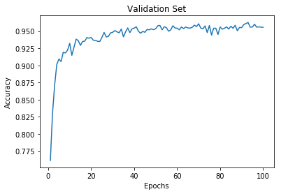
- Epoch iterations 100
I tried increasing the Epoch value to 200, but the model was not improving its accuracy more than 96%, which suggest me to focus my efforts in improving the training dataset and network topology.
- Learning Rate of 0.001
I tried tuning for a smaller learning rate of 0.0001, but the classifier took too long to generalized the model, thus taking too much time in the training phase.
- Batch Size of 128
I tried different values for the batch size, 512, 256, 128 and 64. For my model 128 performed best.
- Optimizer: AdamOptimizer
I did some research about the industry optimizers and the Adam algorithm seems to be a popular choice, since most of the time converge to good models faster than other optimizers. I choose this optimizer for my model, further work needs to be done to evaluate other optimizers.
My final model results were:
- training set accuracy of 0.997
- validation set accuracy of 0.956
- test set accuracy of 0.933
The difference in accuracy between the validation set and the test set is of 0.023%, which is relative small. This suggest the model is generalizing correctly for the unknown test cases.
I started out with the LeNet architecture, without changes this architecture provide me with a model of approximately 80% accuracy.
I ran into some overfitting issues while training the original model, I added dropout regularization in two of the fully connected layers, this allowed to model to better generalized the training set.
I can tell the model is neither underfitting or overfitting, since both the training set and the validation set have high accuracy.
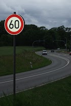
Here are five German traffic signs that I found on the web:
The last image might be difficult to classify speed limits sign have quite a lot of similarity within their class, for example speed limit 60 km/h is similar to speed limit of 80 km/h.
Here are the results of the prediction:
| Image | Prediction |
|---|---|
| Road Work | Road Work |
| Stop | General Caution |
| Yield | Yield |
| Priority Road | Priority Road |
| Speed limit (60 km/h) | Speed limit (60 km/h) |
The model was able to correctly guess 4 of the 5 traffic signs, which gives an accuracy of 80%.
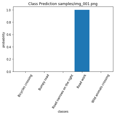
For the first image, the model is really confident that is a road work sign (probability of 0.99), and the image does contain a road work sign. The top five soft max probabilities were:
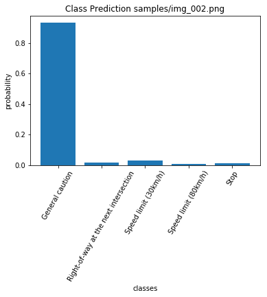
For the second image, the model is confident that is a general caution sign (probability of 0.93), but the actual image is a stop sign. The top five soft max probabilities were:
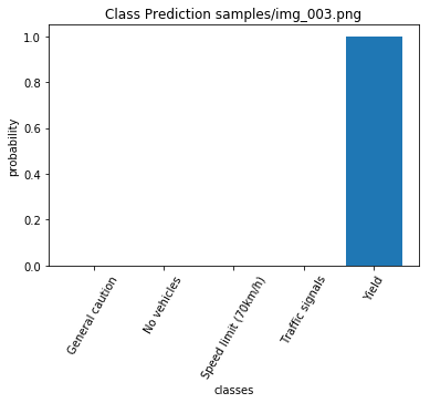
For the third image, the model is really confident that is a yield sign (probability of almost 1.0), and the image does contain a yield sign. The top five soft max probabilities were:
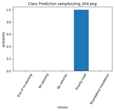
For the fourth image, the model is really confident that is a priority road sign (probability of almost 1.0), and the image does contain a priority road sign. The top five soft max probabilities were:
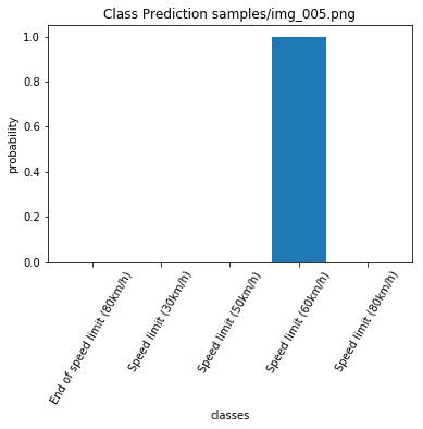
For the fifth image, the model is really confident that is a speed limit 60km/h sign (probability of almost 1.0), and the image does contain a speed limit 60km/h. The top five soft max probabilities were:
