Data and code for “Mapping hormone-regulated cell-cell interaction networks in the human breast at single-cell resolution” (Murrow et al.)
Included is the original code needed to replicate key findings from Murrow et al. Raw FASTQ files, processed gene expression and barcode count matrices, and de-identified patient metadata have been deposited in the Gene Expression Omnibus at accession number GSE198732 and are publicly available as of the date of publication.
Any additional information required to reproduce the data in this study is available from the corresponding authors upon request.
renv::restore()Here, we’ve chosen to read in and plot a subset of the full dataset for speed.
library(Seurat)
library(ggplot2)

source('R/DECIPHER-seq.functions.R')
source('R/DECIPHER-seq.util.R')

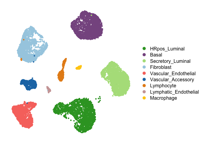
breast.data.sub <- readRDS('Data/breast.data.sub.rds')First, we run consensus iNMF (using the LIGER package) across a range of K values. A heuristic for the maximum value of K for the sweep can be chosen by inspecting PC elbow plots for each cell type. Here, we chose a range of 2 to 40 for all cell types.
library(rliger)
library(RANN)

breast.data <- readRDS('Data/breast.data.rds')
NMF_results <- iNMF_ksweep(breast.data, k.max = 40)
Alternatively, read in the consensus iNMF results from the (entire) processed dataset instead of rerunning the full workflow.
NMF_results <- readRDS('Data/NMF_results.rds')Build phylogenetic trees for K optimization workflow
library(rlist)
library(ape)
library(matrixStats)

phylo_trees <- lapply(NMF_results, build_phylo_tree)
Identify “outlier” activity programs representing rare contaminating cells and plot phylo partitions
program_outlier_score <- lapply(NMF_results, identify_outlier_programs)Choose distance threshold and partition phylogenetic trees
library(patchwork)

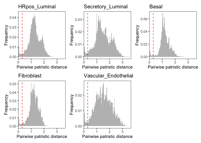
suggested_thresholds = suggest_dist_thresh(phylo_trees)
thresh_use = round(max(suggested_thresholds), 1)
p = plot_hists(phylo_trees, thresh.use = thresh_use)

p[[1]]+p[[3]]+p[[2]]+p[[4]]+p[[5]]library(geiger)
library(igraph)
suggested_thresholds = suggest_dist_thresh(phylo_trees)
thresh_use = round(max(suggested_thresholds), 1)
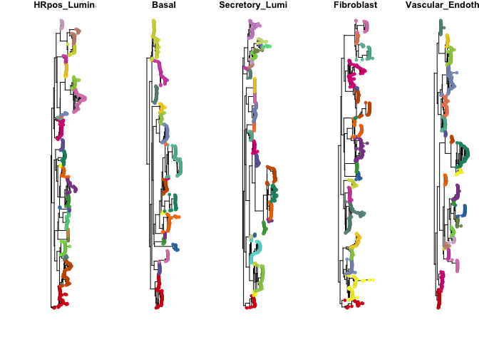
phylo_partitions = mapply(partition_phylo_tree, x = phylo_trees, y = program_outlier_score, dist.thresh = thresh_use, outlier.thresh = 5, SIMPLIFY = F)par(mfrow=c(1,5), mar=c(2.5,5.5,1,1))
plot_phylo_trees(phylo_trees, phylo_partitions)Plot K metric (number of weighted subtrees identified at each choice of NMF rank)
library(dplyr)
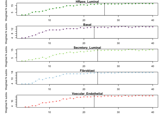
K_metrics = lapply(phylo_partitions, calculate_K_metric)
k.use = lapply(K_metrics, suggest.k)
print(unlist(k.use))
## HRpos_Luminal Basal Secretory_Luminal
## 26 23 24
## Fibroblast Vascular_Endothelial
## 24 23
par(mfrow=c(5,1), mar=c(2.5,5.5,1,1))
for (i in 1:length(K_metrics)){
  plot(2:(dim(K_metrics[[i]])[1]+1), K_metrics[[i]]$weighted_n_subtrees,
       ylab = "Weighted N subtrees", xlab = "NMF Rank K",
       main = names(K_metrics)[i], pch = 16, col = cell_type_cols[i], type = "b")
  abline(v = k.use[[i]])
}
Select NMF results at optimized K values and filter “outlier” programs representing expression in rare cells.
NMF_results_atK <- mapply(FUN = NMF_results_opt_k, NMF_results, k.use, program_outlier_score, SIMPLIFY = F)Calculate the average expression score of each activity program in each sample
metadata <- readRDS('Data/breast.data.metadata.rds')
Expression_score = mapply(NMF_results = NMF_results_atK, metadata = list(metadata), FUN = calc.H.score, SIMPLIFY = F)
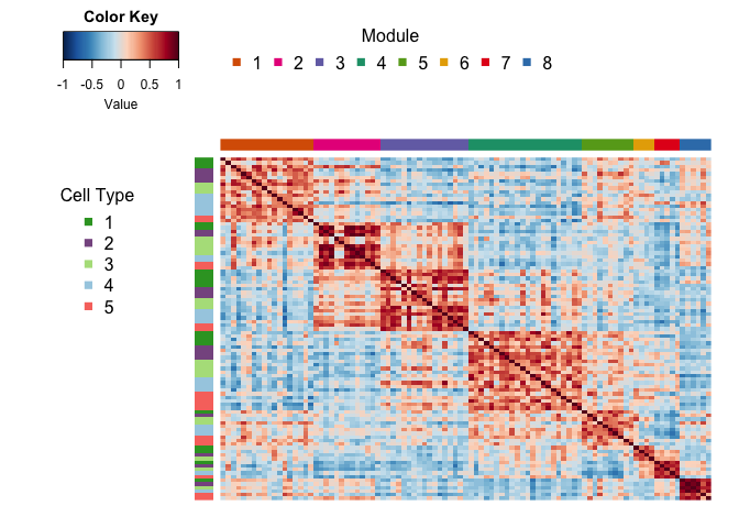
Calculate pairwise Pearson correlations of average sample expression scores for each activity program, perform BCA bootstrap resampling to estimate confidence intervals
source("R/boot.cor.complete.R")
source("R/cor.m.boot.test.R")
library(wBoot)
library(parallel)

Expression_score_cor = cor.m.boot.test(list.cbind(Expression_score), null.hyp = 0, alternative="two.sided")
Expression_score_cor$sig.cor = Expression_score_cor$cor
Expression_score_cor$sig.cor[which(Expression_score_cor$p> 0.05)] = NA
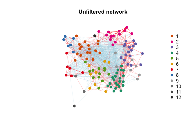
Build weighted network.
Network <- Construct_network(Expression_score_cor)Perform community detection.
library(reticulate)
adjacency_matrix <- Network$mat
py_run_string("import leidenalg as la; import igraph as ig; import numpy as np")
py_run_string("G = ig.Graph.Weighted_Adjacency(r.adjacency_matrix.tolist())")

# sweep across a range of resolutions
py_run_string("optimiser = la.Optimiser()")
py_run_string("profile = optimiser.resolution_profile(G, la.CPMVertexPartition,
        weights = 'weight', resolution_range=(0.001, 0.4), number_iterations = 0)")
sweep = py$profile
modularity = lapply(sweep, function(x){x$modularity})
# Use "resolution" that gives max modularity
partition_use = sweep[[which.max(unlist(modularity))]]
py_run_string("partition = r.partition_use")
py_run_string("diff = optimiser.optimise_partition(partition)")

# Optimise this partition
while(py$diff!=0){
  py_run_string("diff = optimiser.optimise_partition(partition)")
  py_run_string("print(diff)")
}
clustering_res = py$partition
modules = clustering_res$membership + 1
names(modules) = colnames(adjacency_matrix)
Network$modules = modules
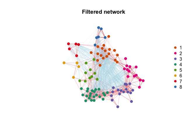
Filter isolated nodes and modules using weighted topological overlap.
library(wTO)
Network <- Filter_network(Network)
Plot results (pre- and post-filtering).
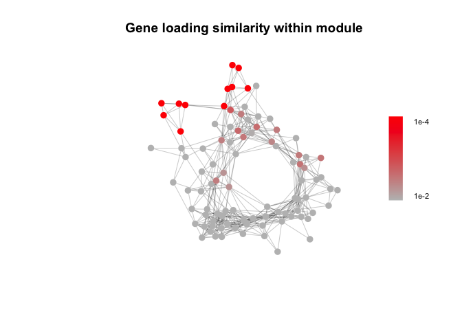
Infer non cell type specific responses, e.g. in response to a shared cue or common microevironment. Non-specific gene signatures (such as artifacts of tissue processing) would also be expected to display similar gene loadings.
gene_correlation_matrix <- Gene_similarity(NMF_results_atK)
gene_similarity_node_pvals <- Permutation_test_gene_cor(Network, gene_correlation_matrix)

edge_weights_fisher = abs(FisherZ(edge.attributes(Network$filtered_network)$weight*edge.attributes(Network$filtered_network)$sign))
plot(Network$filtered_network, layout = Network$filtered_network_coords,
     vertex.color=colorRampPalette(c("grey", "red"))(100)[cut(-log10(gene_similarity_node_pvals), breaks = c(0, seq(-log10(0.01), 4, length.out = 100)))],
     edge.width=0.25, vertex.label.cex=0.5, vertex.size = 7, vertex.label.color="black",
     vertex.label.family="Helvetica", vertex.frame.color=NA, vertex.label.font=2, vertex.label = NA,
     edge.color = c(NA, "grey20")[factor(E(Network$filtered_network)$sign>0)],
     main = "Gene loading similarity within module")
legend_image <- as.raster(matrix(rev(colorRampPalette(c("grey", "red"))(100)), ncol=1))
text(x=1.9, y = c(-0.4,0.4), labels = c("1e-2", "1e-4"), cex = 0.7)
rasterImage(legend_image, 1.55, -0.45, 1.7,0.45)This simplified model does not consider the effects of signal amplification, cooperation between signaling pathways, or higher-order interactions between more than two cell types, but can be used to identify a subset of “high-confidence” direct cell-cell interactions that meet a series of simple criteria. Only test for cell types where the single-cell dataset reflects the tissue composition (e.g. cell types where dissociation artifacts are minimized and sort gates that don’t enrich for one cell type selectively).
library(broom)

interaction_term_res = Infer_direct_interactions(Expression_score, Network, metadata, celltypes.test = c("HRpos_Luminal", "Secretory_Luminal", "Basal"), sort.gate = c("Live_singlet", "Epithelial"))
## Testing direct interactions between cell types: HRpos_Luminal, Secretory_Luminal, Basal
## Testing cells in sort gate: Live_singlet, Epithelial
mat = interaction_term_res$adjacency_matrix
mat[is.na(mat)] = 0
network_directed <- graph_from_adjacency_matrix(t(mat), weighted=T, mode="directed", diag=F)

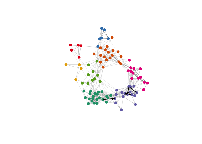
plot.igraph(Network$filtered_network, layout = Network$filtered_network_coords,
            vertex.color=network_module_cols[factor(Network$filtered_modules)],vertex.label = NA,
     edge.width=0.5*edge_weights_fisher, vertex.label.cex=0.5, vertex.size = 7, vertex.label.color="black",
     vertex.label.family="Helvetica", vertex.frame.color=NA, vertex.label.font=2,
     edge.color = c(NA, "grey50")[factor(E(Network$filtered_network)$sign>0)])
plot.igraph(network_directed, layout = Network$filtered_network_coords,
            vertex.color= alpha("black", 0),
            edge.width=2, vertex.label.cex=0.5, vertex.size = 3, vertex.label.color="black",
            vertex.label.family="Helvetica", vertex.frame.color=NA, vertex.label.font=2,
            edge.color = "black",
vertex.label = NA, edge.arrow.size = 0.3, edge.arrow.width = 2, add = T)Identify marker genes statistically associated with each gene program, using ordinary least squares regression of each gene’s normalized (z-scored) expression against the activity program expression score (e.g. cell “expression”) for each program in each cell type, after filtering genes not expressed in that cell type
marker_gene_list <- Marker_gene_analysis(NMF_results_atK, NMF_results)Perform gene set enrichment analysis across activity programs in the DECIPHER-seq network.
library(fgsea)
library(msigdbr)

# Targeted Gene Sets: luteal phase (Pardo et al.) and involution-related (Stein et al.)
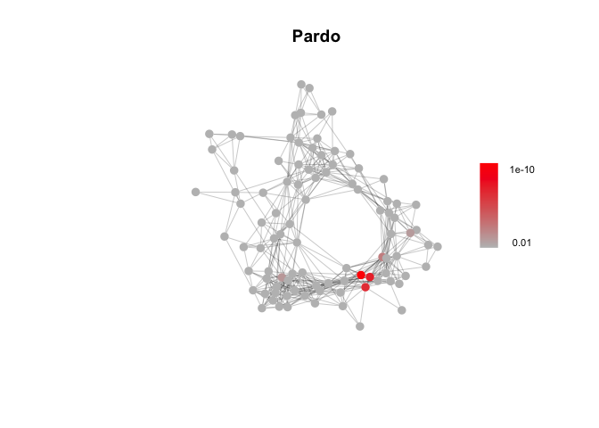
path_list = readRDS('Data/genesets/targeted_pathways.rds')["Pardo"]
Pardo_fgsea_res = fgsea_test(marker_gene_list, Network, path_list)

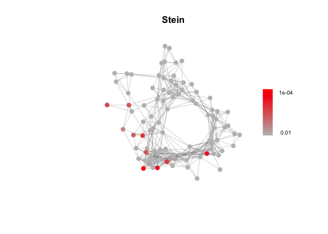
path_list = readRDS('Data/genesets/targeted_pathways.rds')["Stein"]
Stein_fgsea_res = fgsea_test(marker_gene_list, Network, path_list)

# GO Biological Processes
path_df = msigdbr(species = "Homo sapiens", category="C5")
path_df=subset(path_df, gs_subcat%in%c("GO:BP"))
path_list = path_df %>% split(x = .$gene_symbol, f = .$gs_name)
GO_BP_fgsea_res = fgsea_test(marker_gene_list, Network, path_list)

# Hallmark Gene Sets
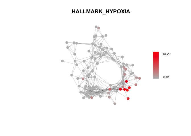
path_df = msigdbr(species = "Homo sapiens", category="H")
path_list = path_df %>% split(x = .$gene_symbol, f = .$gs_name)
Hallmark_fgsea_res = fgsea_test(marker_gene_list, Network, path_list)
Plot enrichment of selected gene sets.
# A few example plots
plot_fgsea(Network, Pardo_fgsea_res, "Pardo", fdr_min = 1e-10)plot_fgsea(Network, Stein_fgsea_res, "Stein", fdr_min = 1e-4)plot_fgsea(Network, Hallmark_fgsea_res, "HALLMARK_HYPOXIA", fdr_min = 1e-20)Identify gene sets enriched across modules in the DECIPHER-seq network.
# choose gene sets to test
sets_to_test = rbind(Stein_fgsea_res, Pardo_fgsea_res, GO_BP_fgsea_res, Hallmark_fgsea_res)

enrichment_pval = Get_enrichment_pvals(sets_to_test, Network)
## GOBP_CIRCULATORY_SYSTEM_DEVELOPMENT
## 9.999e-05
## GOBP_POSITIVE_REGULATION_OF_PEPTIDYL_TYROSINE_PHOSPHORYLATION
## 9.999e-05
## GOBP_PYRUVATE_METABOLIC_PROCESS
## 9.999e-05
## GOBP_REGULATION_OF_PEPTIDYL_TYROSINE_PHOSPHORYLATION
## 9.999e-05
## GOBP_TISSUE_REMODELING
## 9.999e-05
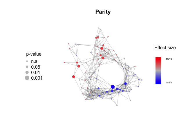
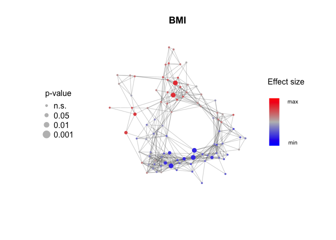
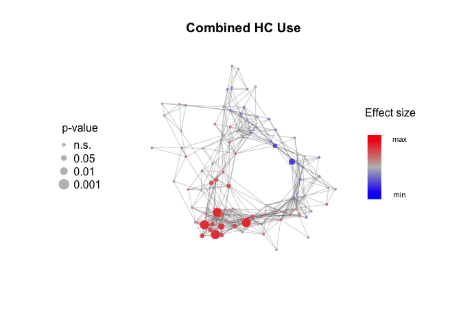
Measure the effect size and p-values for association with metadata features. Mann-Whitney test and Wilcoxon effect size (r) for binary features, linear regression and Pearson correlation (r) for continuous features.
library(rstatix)

# for binary variables, create a metadata column with only two levels
metadata$Parity.Y.N[metadata$Parity.Y.N=="unknown"] = NA
metadata$Parity.Y.N = factor(metadata$Parity.Y.N, levels = c("yes", "no"))
Parity_effect_size = Calculate_metadata_associations(Network, Expression_score, metadata, feature.to.test = "Parity.Y.N", type = "binary")

BMI_effect_size = Calculate_metadata_associations(Network, Expression_score, metadata, feature.to.test = "BMI", type = "continuous")
## Warning in Calculate_metadata_associations(Network, Expression_score,
## metadata, : Converting metadata feature.to.test to continuous variable
metadata$HC_use[metadata$HC_use=="progestin"] = NA
metadata$HC_use = factor(metadata$HC_use, levels = c("combined", "none"))
HC_use_effect_size = Calculate_metadata_associations(Network, Expression_score, metadata, feature.to.test = "HC_use", type = "binary")Plot_metadata_association(Network, Parity_effect_size, plot.title = "Parity")Plot_metadata_association(Network, BMI_effect_size, plot.title = "BMI")Plot_metadata_association(Network, HC_use_effect_size, plot.title = "Combined HC Use")