rate:

Reliable Analytic Thermochemical Equilibrium

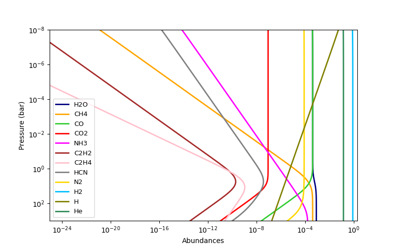
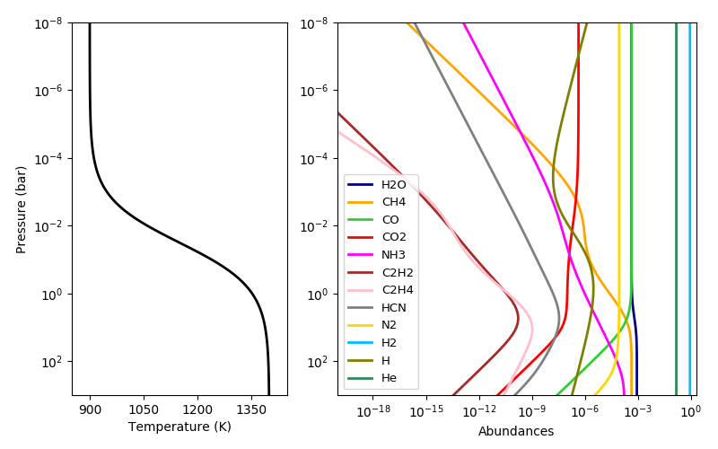
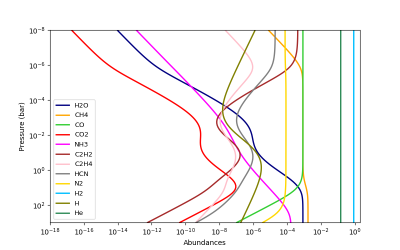
This code computes thermochemical-equilibrium abundances for a H-C-N-O system with known pressure, temperature, and elemental abundances. The output abundances are H2O, CH4, CO, CO2, NH3, C2H2, C2H4, HCN, and N2, H2, H, and He.

These calculations are valid over:

pressures from 10^-8 to 10³ bar,
temperatures from 200 to ~2000 K,
C-N-O elemental abundances from 10^-3 to 10² times solar abundances in hydrogen-dominated systems.

Team Members
Install
Getting Started
Be Kind
License

Team Members

Patricio Cubillos (IWF) patricio.cubillos@oeaw.ac.at
Jasmina Blecic (NYU Abu Dhabi)
Ian Dobbs-Dixon (NYU Abu Dhabi)

Install

rate is compatible with both Python2 and Python3, and runs (at least) in both Linux and OSX.
To obtain the rate code, clone this repository to your local machine with the following terminal commands:

# Clone the repository to your working directory:  
git clone https://github.com/pcubillos/rate/

Getting Started

The following Python script shows how to compute equilibrium abundances with rate:

import numpy as np
import matplotlib.pyplot as plt
# Make sure to have/add the path to the rate package in your pythonpath:
import rate

# Initialize object with solar composition:
r = rate.Rate(C=2.5e-4, N=1.0e-4, O=5.0e-4, fHe=0.0851)

# Define atmospheric profile:
nlayers = 100
press = np.logspace(-8, 3, nlayers)  # bars
temp1 = np.tile(1400.0, nlayers)     # kelvin

# Compute abundances:
Q1 = r.solve(temp1, press)

# See results:
labels = r.species
cols   = ["navy", "orange", "limegreen", "red",         "magenta", "brown",
          "pink", "0.5",    "gold",      "deepskyblue", "olive",    "seagreen"]

plt.figure(-1, (8,5))
plt.clf()
for q, col, lab in zip(Q1, cols, labels):
  plt.loglog(q, press, lw=2, color=col, label=lab)
plt.ylim(np.amax(press), np.amin(press))
plt.legend(loc="lower left", fontsize=9.5)
plt.xlim(1e-25, 2)
plt.xlabel("Abundances")
plt.ylabel("Pressure (bar)")
plt.xticks(np.logspace(-24, 0, 7))

# A 'more interesting' temperature profile:
temp2 = 900+500/(1+np.exp(-(np.log10(press)+1.5)*1.5))
Q2 = r.solve(temp2, press)

plt.figure(-2, (8,5))
plt.clf()
ax = plt.axes([0.1, 0.12, 0.3, 0.83])
plt.semilogy(temp2, press, lw=2, color="k")
plt.ylim(np.amax(press), np.amin(press))
plt.xlim(850, 1450)
ax.set_xticks([900, 1050, 1200, 1350])
plt.ylabel("Pressure (bar)")
plt.xlabel("Temperature (K)")
ax = plt.axes([0.47, 0.12, 0.5, 0.83])
for q, col, lab in zip(Q2, cols, labels):
  plt.loglog(q, press, lw=2, color=col, label=lab)
plt.ylim(np.amax(press), np.amin(press))
plt.xlim(1e-20, 2)
plt.xticks(np.logspace(-18, 0, 7))
plt.legend(loc="lower left", fontsize=9.5)
plt.xlabel("Abundances")

# A carbon-dominated atmosphere, same temperature as before:
Q3 = r.solve(temp2, press, C=1e-3)
plt.figure(-3, (8,5))
plt.clf()
for q, col, lab in zip(Q3, cols, labels):
  plt.loglog(q, press, lw=2, color=col, label=lab)
plt.ylim(np.amax(press), np.amin(press))
plt.legend(loc="lower left", fontsize=9.5)
plt.xlim(1e-18, 2)
plt.xlabel("Abundances")
plt.ylabel("Pressure (bar)")

Be Kind

Please, be kind and acknowledge the effort of the authors by citing the article associated to this project:

Cubillos, Blecic, & Dobbs-Dixon (2019): Towards More Reliable Analytic Thermochemical-equilibrium Abundances, ApJ, 872, 111.

pcubillos/rate