Geometric Multigrid

High speed Geometric Multigrid solver in pure Julia.


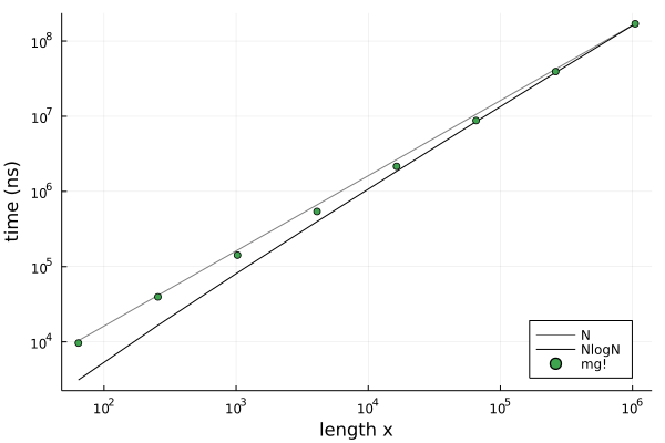
Benchmark example for `mg!` solver demonstrating approximately linear solution time scaling with the length of the solution vector.

Usage

Define a matrix and solution

julia> using GeometricMultigrid

julia> function setup_2D(n=128,T::Type=Float64)
           L = zeros(T,n+2,n+2,2); L[3:n+1,2:n+1,1] .= 1; L[2:n+1,3:n+1,2] .= 1; 
           x = T[i-1 for i ∈ 1:n+2, j ∈ 1:n+2]
           Poisson(L),FieldVector(x)
       end

julia> A,x = setup_2D(4);

Define the source term and solve.

julia> b = A*x;

julia> y,it = mg(A,b);

julia> print("number of iterations=",it)
number of iterations=6

julia> y
16-element FieldVector{Float64, 2, Matrix{Float64}}:
 -1.487754625809229
 -0.48775463361508725
  0.5122453605258042
  1.5122453584556865
 -1.4877546258567003
  ⋮
  1.5122453627041033
 -1.487754626187825
 -0.4877546300066085
  0.512245365911722
  1.5122453643079126

Check solution

julia> A*y ≈ b
true

To use the in-place version, you need to set up a multi-grid SolveState

julia> st = mg_state(A,zero(x),b)
SolveState{Float64}:
   residual=2.8284271247461903
   residual=0.0
   nothing

This shows the residual on each level of the grid. Since there are only 4-grid points in each dimension, the grid can only be resitricted once. Restricting further to a 1x1 grid would produce the singular equation 0*x=b.

The system can now be solved in-place without further allocation:

julia> @allocated mg!(st)
0

julia> st
SolveState{Float64}:
   residual=1.5436920360020765e-8
   residual=2.335855716890062e-16
   nothing

julia> st.x
16-element FieldVector{Float64, 2, Matrix{Float64}}:
 -1.487754625809229
 -0.48775463361508725
  0.5122453605258042
  1.5122453584556865
 -1.4877546258567003
  ⋮
  1.5122453627041033
 -1.487754626187825
 -0.4877546300066085
  0.512245365911722
  1.5122453643079126

Method

Geometric multigrid methods use a recursive approach to solve linear algebra problems stemming from partial differential equations posed on a structured numerical grid. Algebraic multigrid methods apply to a broader class of problems, but are typically not as fast as Geometric Multigrid when applicable.

The problem on the fine grid is restricted down to a coarsened grid, which is therefore faster to solve, and the solution is prolongated back up to the fine grid where any remaining high-frequency errors are smoothed. In this package the coarse grid is simply half the size in every dimension, the restriction operation is a sum over the local points and prolongation is a copy back up to those points. This is done recursively until halving is no longer possible, and then the solution is prolongated all the way back up to the top level in a process called a V-cycle. The default smoother is 3 iterations of the Gauss-Sidel method. The benchmark plot above shows this results in solution time with approximately linear scaling with the vector length.

Implementation

Geometric Multigrid methods make use of the regular spatial connectivity of the grid to define the restriction and prolongation operators. These concepts are built into the package using the FieldVector type, which is simply a wrapper around a multi-dimensional array.

julia> _,x = setup_2D(3);

julia> x
9-element FieldVector{Float64, 2, Matrix{Float64}}:
 1.0
 2.0
 3.0
 1.0
 2.0
 3.0
 1.0
 2.0
 3.0

julia> x.data
5×5 Matrix{Float64}:
 0.0  0.0  0.0  0.0  0.0
 1.0  1.0  1.0  1.0  1.0
 2.0  2.0  2.0  2.0  2.0
 3.0  3.0  3.0  3.0  3.0
 4.0  4.0  4.0  4.0  4.0

julia> x.R
3×3 CartesianIndices{2, Tuple{UnitRange{Int64}, UnitRange{Int64}}}:
 CartesianIndex(2, 2)  CartesianIndex(2, 3)  CartesianIndex(2, 4)
 CartesianIndex(3, 2)  CartesianIndex(3, 3)  CartesianIndex(3, 4)
 CartesianIndex(4, 2)  CartesianIndex(4, 3)  CartesianIndex(4, 4)

julia> norm(x,Inf)  # does not include buffer elements in x.data
3.0

The R field holds the CartesianIndices range of the points in the field excluding any buffer elements, with the default being a buffer layer 1-element thick on all boundaries. Note that a FieldVector acts like a 1D vector by default, despite the underlying multidimensional data and buffer. This allows general linear algebra functions to be applied, as shown above.

The extension of FieldVectors to matrices is the FieldMatrix type. Currently, this type only defines symmetric matrices with M=length(dims) subdiagonals held in an M+1 dimensional array L. The Poisson function builds a matrix from L with zero-sum rows, which is a requirement for conservative Poisson equations: ∫ ∇⋅β∇ϕ dv = ∮ β ∂ϕ/∂n da.

julia> A,_ = setup_2D(3);

julia> A
9×9 FieldMatrix{Float64, 2, Array{Float64, 3}, Matrix{Float64}}:
 -2.0   1.0   0.0   1.0   0.0   0.0   0.0   0.0   0.0
  1.0  -3.0   1.0   0.0   1.0   0.0   0.0   0.0   0.0
  0.0   1.0  -2.0   0.0   0.0   1.0   0.0   0.0   0.0
  1.0   0.0   0.0  -3.0   1.0   0.0   1.0   0.0   0.0
  0.0   1.0   0.0   1.0  -4.0   1.0   0.0   1.0   0.0
  0.0   0.0   1.0   0.0   1.0  -3.0   0.0   0.0   1.0
  0.0   0.0   0.0   1.0   0.0   0.0  -2.0   1.0   0.0
  0.0   0.0   0.0   0.0   1.0   0.0   1.0  -3.0   1.0
  0.0   0.0   0.0   0.0   0.0   1.0   0.0   1.0  -2.0

julia> diag(A).data
5×5 Matrix{Float64}:
 0.0   0.0   0.0   0.0  0.0
 0.0  -2.0  -3.0  -2.0  0.0
 0.0  -3.0  -4.0  -3.0  0.0
 0.0  -2.0  -3.0  -2.0  0.0
 0.0   0.0   0.0   0.0  0.0

julia> eigen(A).values
9-element Vector{Float64}:
 -5.999999999999996
 -3.999999999999999
 -3.999999999999995
 -3.000000000000001
 -3.0
 -2.0000000000000018
 -0.9999999999999999
 -0.9999999999999986
  5.551115175576828e-16

Again, this wrapper allows familiar linear algebra functions to be used, without losing the underlying geometric structure of the data. Fast custom linear algebra functions are defined for norm(x), dot(x,b), dot(x,A,b), mul!(b,A,x) and *.

Finally the SolveState is a recursive type which holds the required arrays for the mg! function.

peteryim/GeometricMultigrid.jl

Geometric Multigrid

Usage

Method

Implementation