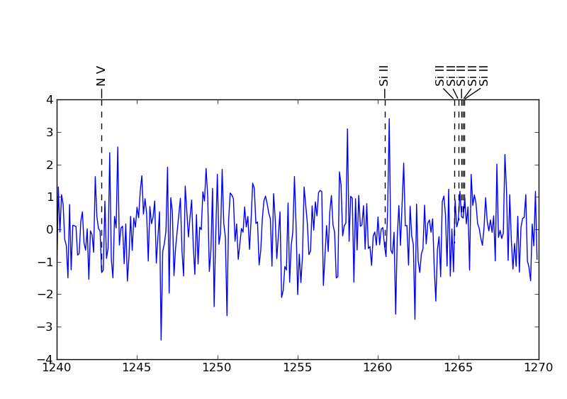
Manually labeling features in a crowed plot can be very time consuming. Functions in this module can be used to automatically place labels without the labels overlapping each other. This is useful, for example, in creating plots of a spectrum with spectral lines identified with labels.
For more details see http://lineid-plot.readthedocs.io.
Use pip:
$ pip install lineid_plot
Detailed examples are provided at http://lineid-plot.readthedocs.io .
A basic plot can be created by calling the function
plot_line_ids(), and passing labels and x-axis locations of
features.
>>> import numpy as np
>>> from matplotlib import pyplot as plt
>>> import lineid_plot

>>> wave = 1240 + np.arange(300) * 0.1
>>> flux = np.random.normal(size=300)

>>> line_wave = [1242.80, 1260.42, 1264.74, 1265.00, 1265.2, 1265.3, 1265.35]
>>> line_label1 = ['N V', 'Si II', 'Si II', 'Si II', 'Si II', 'Si II', 'Si II']

>>> lineid_plot.plot_line_ids(wave, flux, line_wave, line_label1)
>>> plt.show()
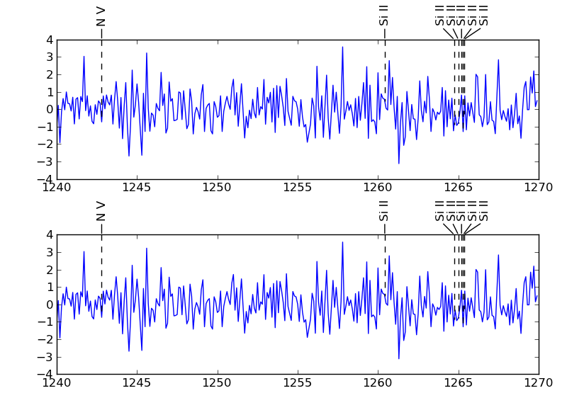
The plot_line_ids() function also accepts Axes and/or Figure
instances where labels are to be draw.
>>> import numpy as np
>>> from matplotlib import pyplot as plt
>>> import lineid_plot

>>> wave = 1240 + np.arange(300) * 0.1
>>> flux = np.random.normal(size=300)
>>> line_wave = [1242.80, 1260.42, 1264.74, 1265.00, 1265.2, 1265.3, 1265.35]
>>> line_flux = np.interp(line_wave, wave, flux)
>>> line_label1 = ['N V', 'Si II', 'Si II', 'Si II', 'Si II', 'Si II', 'Si II']
>>> label1_sizes = np.array([12, 12, 12, 12, 12, 12, 12])

>>> fig = plt.figure(1)

>>> ax = fig.add_axes([0.1,0.06, 0.85, 0.35])
>>> ax.plot(wave, flux)
>>> lineid_plot.plot_line_ids(wave, flux, line_wave, line_label1, ax=ax)

>>> ax1 = fig.add_axes([0.1, 0.55, 0.85, 0.35])
>>> ax1.plot(wave, flux)
>>> lineid_plot.plot_line_ids(wave, flux, line_wave, line_label1, ax=ax1)
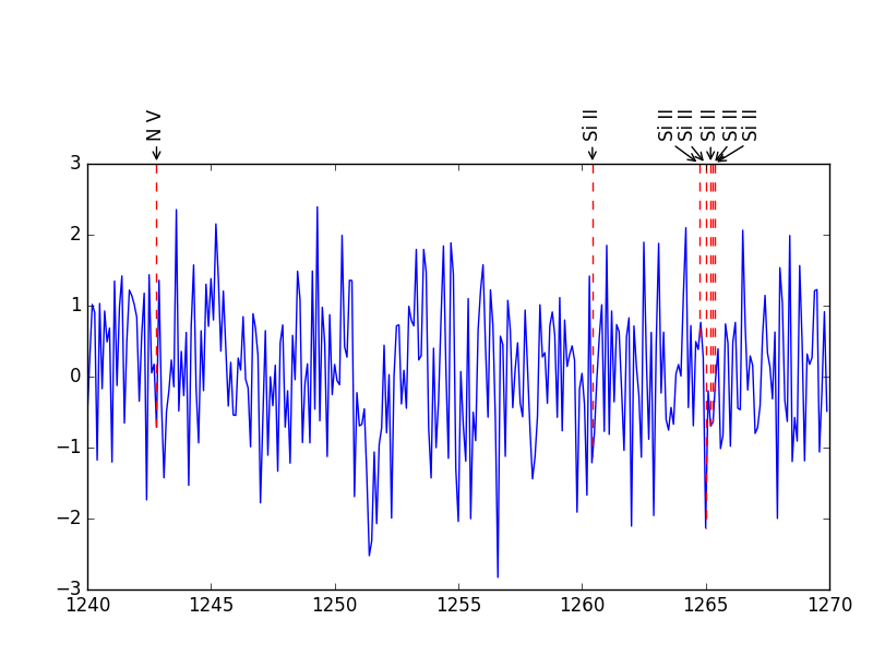
The label text and the short line extending down from the text are created using
the annotate method of a matplotlib Axes object. The longer line extending
down to a point in the spectrum is created using the plot method on a
matplotlib Axes instance. The plot_line_ids function accepts keywords to
pass directly to these methods, annotate_kwargs and plot_kwargs,
respectively. But the best method for customizing boxes and lines is by
obtaining a reference to it as shown in another example below.
>>> import numpy as np
>>> from matplotlib import pyplot as plt
>>> import lineid_plot

>>> wave = 1240 + np.arange(300) * 0.1
>>> flux = np.random.normal(size=300)

>>> line_wave = [1242.80, 1260.42, 1264.74, 1265.00, 1265.2, 1265.3, 1265.35]
>>> line_label1 = ['N V', 'Si II', 'Si II', 'Si II', 'Si II', 'Si II', 'Si II']

>>> ak = lineid_plot.initial_annotate_kwargs()
>>> ak
{'arrowprops': {'arrowstyle': '->', 'relpos': (0.5, 0.0)},
 'horizontalalignment': 'center',
 'rotation': 90,
 'textcoords': 'data',
 'verticalalignment': 'center',
 'xycoords': 'data'}
>>> ak['arrowprops']['arrowstyle'] = "->"

>>> pk = lineid_plot.initial_plot_kwargs()
>>> pk
{'color': 'k', 'linestyle': '--'}
>>> pk['color'] = "red"

>>> lineid_plot.plot_line_ids(wave, flux, line_wave, line_label1, annotate_kwargs=ak, plot_kwargs=pk)
>>> plt.show()
The boxes and the lines extending to the flux level both have their label set to a unique value. If the input contains identical labels then the function will construct unique lables by appending text. These can be used to quickly identify them.
>>> for i in ax.texts:
   ....:     print i.get_label()
   ....:
N V
Si II_num_1
Si II_num_2
Si II_num_3
Si II_num_4
Si II_num_5
Si II_num_6
>>> for i in ax.lines:
   ....:     print i.get_label()
   ....:
_line0
N V_line
Si II_num_1_line
Si II_num_2_line
Si II_num_3_line
Si II_num_4_line
Si II_num_5_line
Si II_num_6_line
The label _line0 corresponds to the data plot and was assigned by
Matplotlib.
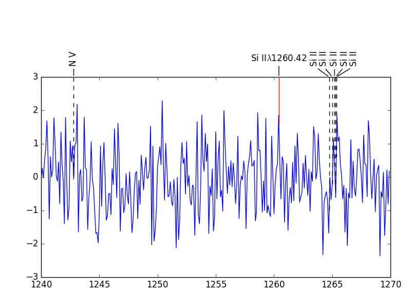
We can get a reference to an annotation box or a line using the Axes.findobj
method. Once we get a reference we can change its properties. This is the best
method for customizing boxes and lines.
>>> import numpy as np
>>> from matplotlib import pyplot as plt
>>> import lineid_plot

>>> wave = 1240 + np.arange(300) * 0.1
>>> flux = np.random.normal(size=300)

>>> line_wave = [1242.80, 1260.42, 1264.74, 1265.00, 1265.2, 1265.3, 1265.35]
>>> line_label1 = ['N V', 'Si II', 'Si II', 'Si II', 'Si II', 'Si II', 'Si II']

>>> fig, ax = lineid_plot.plot_line_ids(wave, flux, line_wave, line_label1)

>>> b = ax.findobj(match=lambda x: x.get_label() == 'Si II_num_1')[0]
>>> b.set_rotation(0)
>>> b.set_text("Si II$\lambda$1260.42")

>>> line = ax.findobj(match=lambda x: x.get_label() == 'Si II_num_1_line')[0]
>>> line.set_color("red")
>>> line.set_linestyle("-")

>>> plt.show()
Adding a label to lines can cause problems when using plt.legend(): the
legend will include the lines drawn from text box to spectrum location. There
are two ways of overcoming this. First is to provide explicit artists and texts
to plt.legend(). Second is to tell lineid_plot not to add these labels
by passing in add_label_to_artists=False. Of-course, if we use the second
option then we can't use the above method for finding text and lines.
fig, ax = lineid_plot.plot_line_ids(
    wave, flux, line_wave, line_label1, max_iter=300, add_label_to_artists=False
)The placements are calculated using a simple, iterative algorithm adapted from the procedure lineid_plot in the NASA IDL Astronomy User's Library. Matplotlib makes most of the other computations, such as extracting width of label boxes, re-positioning them etc., very easy.
The main function in the module is plot_line_ids(). Labeled plots can be
created by passing the x and y coordinates, for example wavelength and flux,
along with the x coordinates of the features and their labels. The x coordinates
are adjusted until the labels, of given size, do not overlap, or when the
iteration limit is reached.
Users can provide the Axes instance or the Figure instance on which plots are to be made. If an Axes instance is provided, then the data is not plotted; only the labels are marked. This allows the user to separate plotting from labeling. For example, the user can create multiple Axes on a figure and then pass the Axes on which labels are to be marked. No changes are made to the existing layout.
The labels and a short line for each label are create using matplotlib's
Axes.annotate method. The longer lines extending down into the plot are
created using matplotlib's Axes.plot method.
The y axis locations of labels and annotation points i.e., arrow tips, can also
be passed to the plot_line_ids() function. Minor changes can be passed using
the box_axes_space keyword, where as major changes can be passed using the
arrow_tip and box_loc keywords. The former is in figure fraction units
and the latter two are in data coordinates. The latter two can be specified
separately for each label. This is very useful in crowded regions. These
features along with the ability to pass an Axes instance gives the program a lot
of flexibility.
An extension line from the annotation point to the y data value at the location
of the identification i.e., flux level at the line, is drawn by default. The
flux at the line is calculated using linear interpolation. This can be turned
off using the extend keyword. This keyword can be set separately for each
feature.
The boxes containing text label and the line extending down can be customized by
paasing annotate_kwargs and plot_kwargs respectively. Use
initial_annotate_kwargs() and initial_plot_kwargs() to obtain the
default dictionaries used. We can customize these dictionaries and pass them to
plot_line_ids. Further customizations can be performed by obtaining a
reference to the annotation or line and using the matplotlib API.
The plot_line_ids() function returns the Figure and Axes instances used.
Additional customizations, such as manual adjustments to positions, can be
carried out using these references. To easily identify the ojects, each label
box and extension line have its label property set to a string that depends
on the label text provided. Identifying the Matplotlib objects corresponding to
these and customizing them are made easy by the many features provided by
Matplotlib.
The maximum number of iterations to use while calculating label positions can be
supplied using the max_iter keyword. The amount of adjustment to be made in
each iteration and when to change the adjustment factor can also be supplied.
The defaults for these should be enough for most cases.
Released under BSD; see http://www.opensource.org/licenses/bsd-license.php.
Code here is adapted from lineid_plot procedure in the IDL Astronomy User's Library (IDLASTRO) IDL code distributed by NASA.
For comments and suggestions, email to user prasanthhn in the gmail.com domain.


