MSc project - 3D Human Pose and Shape Estimation

Overview

This is the Github repository of my MSc Thesis in Computational Statistics and Machine Learning at University College London. The thesis aims at expanding on the work by Rhodin et al in the paper Unsupervised Geometry-Aware Representation for 3D Human Pose Estimation (https://arxiv.org/pdf/1804.01110.pdf). Here we provide an overview of the work done, more details can be found in my dissertation.

I will be trying to be as faithful as possible to the work done without "embellishing" the results as seems to be common practice in the research community. I will also keep a very informal tone, otherwise reading this would be super boring - thanks for getting this far by the way. After all I am not trying to get funding or anything like that. Ok getting serious now.

This works is divided in two parts:

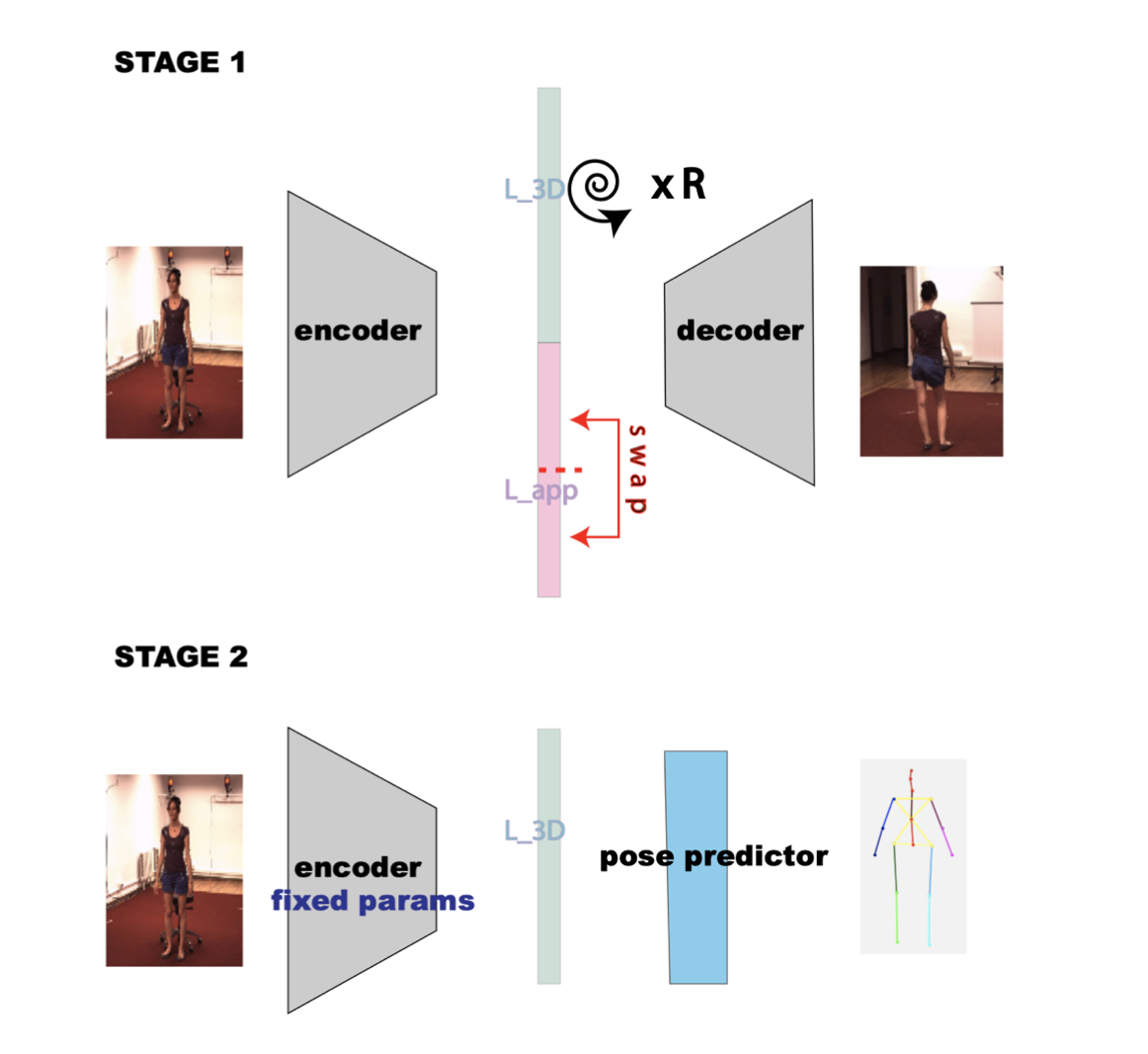
Reproducing the work from Rhodin that leverages multiple cameras at training time to estimate the 3D pose from monocular images. This is done by training an encoder-decoder architecture to reproduce images from different angles given an in input image. In the first stage, the encoder-decoder is trained on the multiple views by feeding as input image, the image from a different camera and the 3D rotation between the root joints in the two images. In the second stage, the weights of the encoder are fixed and a shallow network is trained on top of the encoder to minimise the L2 distance between the outputs and the 3D joints. With this protocol, we can reduce the pose data needed to solve the regression problem with an error reported below - More details on the original paper (https://arxiv.org/pdf/1804.01110.pdf).

Figure 1: Training stages of the architecture by Rhodin at al. In stage 1, we train on predicting the image from a different camera. In stage 2, we train on predicting the 3D pose.

2) Expand on the work done by Rhodin and learn pose and shape parameters of the SMPL model (https://smpl.is.tue.mpg.de/) which is a realistic body model. As there are no ground truths available, we devise a training protocol that exploits: the 3D joints location, the silhouettes images present in the dataset and a prior for the body model parameters.

After training the encoder the same way as in 1) we also train a GAN on realistic pose and shape parameters (θ and β below) of the SMPL model using data from the SURREAL dataset (https://www.di.ens.fr/willow/research/surreal/data/). After training, we will discard the generator and only use the discriminator. In the body model estimation the weights of the discriminator will be fixed and the loss of the discriminator will act as a regulariser constraining the SMPL parameters to be realistic.

Then we construct the final network as in the image below. The network aims to minimise a linear combination of three losses:

L_pose: the loss distance between the joints of the SMPL model and the ground truths (available in the dataset).
L_verts: the loss between the rasterised vertices and the ground truth silhouettes (available in the dataset).
L_gan: the loss on the SMPL parameters θ and β which acts as a regulariser in SMPL parameters space (trained previously).

Same as before, only the 3D poses from subject 1 were used.

Figure 2: Diagram of the architecture blocks used in the body model prediction from monocular images. At training time we leverage the silhouttes and a discriminator previously trained on the allowed poses and the encoder previously trained. The whole architecture is differentiable (including the resteriser - https://arxiv.org/abs/1711.07566 and the SMPL model).

Results

The encoder-decoder architecture was trained on images subjects 1,3,5,7 but the pose regressor and the SMPL parameters regressor only leveraged the 3D poses of 1 subject (subject 1). Our 3D pose architecture yield comparable results to Rhodin's results. One key difference between our approach and Rhodin's is that we most likely used different augmentations (the angle for the in-plane rotations was not reported in Rhodin's approach). Therefore, our approach might be more stable to poses at different angle although the N-MPJ on the test set is higher (152 mm vs 146 mm). NA means that the value was not reported in the paper. The results of the Mean per Joint Error (MPJ), Normalised MPJ and Procustes Aligned MPJ is reported above.

Figure 3: Quantitative results from the 3D joints prediction task.

Regarding the results from the SMPL parameters regressor we aren't able to provide quantitative results because the ground truth SMPL parameters for the human3.6M were not available during this research. However we can provide qualitative examples. Below we see two predictions from the monocular images from the test set. In the first picture the shape and pose of the person appears correctly (at least through visual inspection), while in the second picture it appears distorted. This is ikely to happen because in the first picture the subject is facing the camera which is a pose closer to the zero pose (subject facing the camera in resting pose). In the second picture the subject is facing away from the camera so the resulting prediction requires a 180 degrees rotation from the rest pose. In these cases the L_verts and L_pose optimisation take over the L_gan loss optimisation so the poses produced look unrealistic. This is due to the uncontrained nature of the SMPL parameters prediction, especially by three issues:

There is a mismatch between the 3D pose points used in the H3.6M dataset and the 3D pose point of the SMPL model. this means that the hip-joints could not be used as ground truths. These joints are vital to make sure that the predicted poses have correct orientation.
The SMPL parameters are inherently unconstrained. Linear blend skinning of the SMPL model gives good vertices location when the blended transformations are not very different. However we might have issues if we need to blend transformations that are very far from one another in their rotation component. These large rotations are not uncommon in the human body because shoulders, wrists, or even elbows exhibit a rather large range of motion. As a consequence, the linear blending formulation is inherently unconstrained and can generate unrealistic shapes given by extreme joints rotation.
The vertex prediction is unconstrained. Projecting the vertices over 4 masks is an heavily unconstrained supervised problem.

In spite of these three issues, these results look promising and show that the SMPL paramterers prediction might be possible even when only leveraging poses from one subject. This was never attempted before in the literature (at least to our knowledge). A better balancing of the losses or modifying the initialisation of the base pose and shape could mitigate the issue presented above.

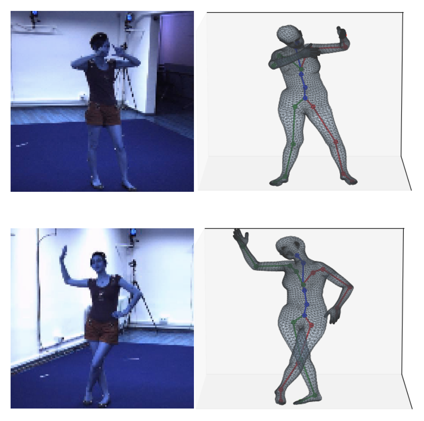
Figure 4: Two examples of input^* and output from the SMPL model regressor architecture. The predictions seem reasonable, although with a few imperfections (position of the head).

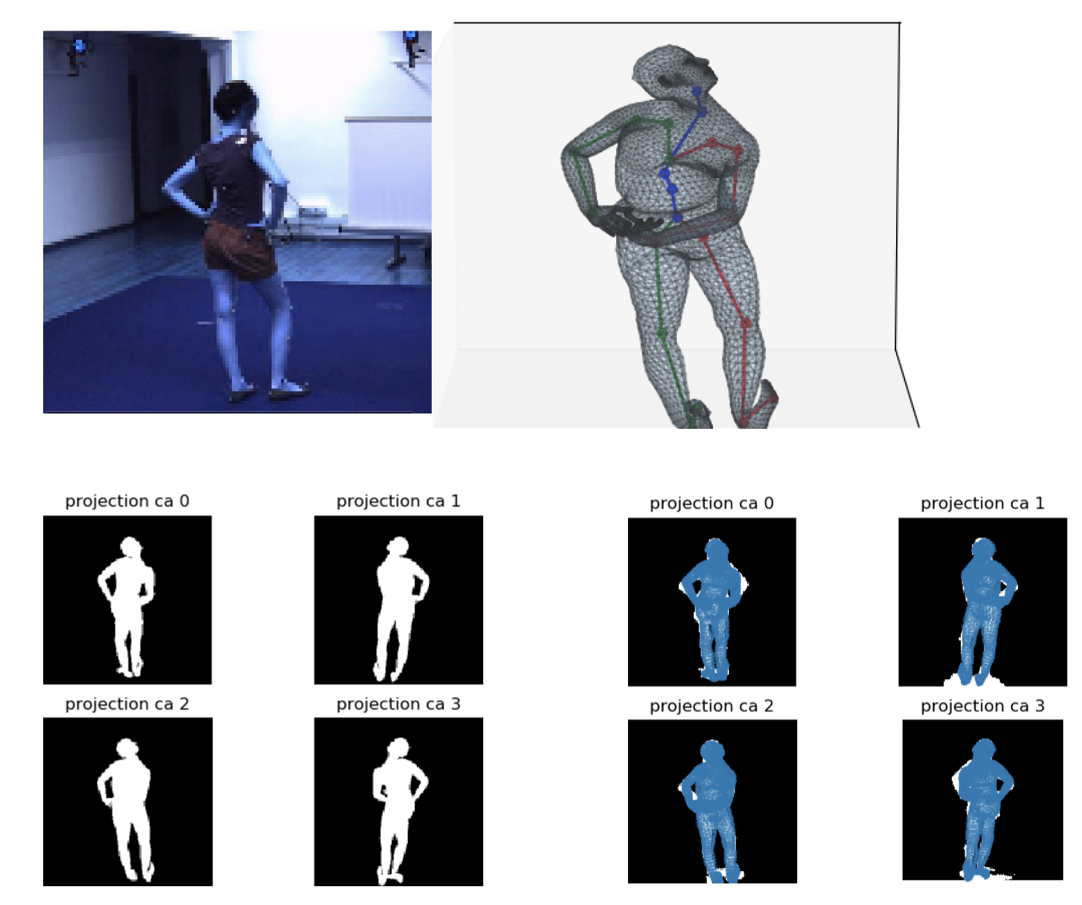
Figure 5: Figure 4: One example of input^* and output from the SMPL model regressor architecture. The prediction here is off most likely for the reasons explained above.

^* I apologised for the bluish images, here the RGB color were messed up when I was getting this the night before my thesis submission. I didn't realise because I set up a blue light on my screen (I know, hilarious).

Further Discussion and Limitation

The approach used here is not directly applicable to a real-world scenario for several reasons:

At training time, in addition to assuming the use of 4 calibrated cameras, during the encoder decoder training we assume that we know the location of the root joint for each subject. This is effectvely cheating as we simplify the problem and actually I believe that the encoder-decoder architecture can only work with this assumption. By taking the rotation between the root joints in the two input images (and not just the rotation between the two cameras) we have a much wider of range of rotations since the subjects are moving in the picture. Therefore it would effectively be like we are leveraging data from more than the 4 views available.
Real time prediction is really slow as we are optimising to use as little data as possible.
In a real world application, we would like an approach that does not exploit sensors since they create a bias in the input image. In addition we would need some form of data in the wild, augmenting the images or anything to reduce domain variance for this to work in the real world.
Getting more supervised data would make a much more accurate model.

Thanks for reading!

Usage

Setup - Python 3.6

Download Python 3.7 and install requirements. Additional requirements that might have to be installed manually are:
- SMPL model (Download the SMPL model files here. Here we use the neutral model
- Install all the prerequisites. This can be done using the command:
```
 conda create --name ** ENV_NAME ** --file requirements.txt
```
This will not install packages installed using pip so you might need to do:
```
     pip install chumpy    #used for the SMPL model

     pip install neural-renderer-pytorch
```
Alternatively you can recreate the environment from requirements.yml, although that will give an error when encountering the pip packages

The neural rendering package is an implementation of the paper Neural 3D Mesh Rende (http://hiroharu-kato.com/projects_en/neural_renderer.html). The implementation used can be found on the github page https://github.com/daniilidis-group/neural_renderer.

Note that this package requires a GPU to be run, while everything else can be run on the cpu.
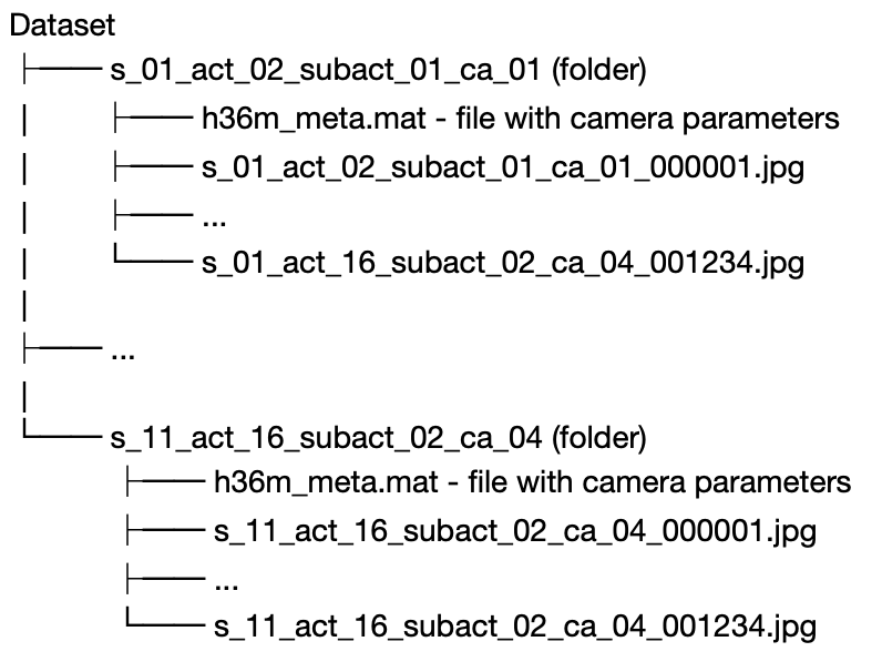
Download Human 3.6 M dataset (http://vision.imar.ro/human3.6m/description.php). Here explain the arrangement of data. The dataset should be arranged as follows:

where "s" denotes the subject, "act" the act, "subact" the subatct, "ca" the camera and the number the frames. place the dataset in the data folder.

Download the Masks. These should be arranged the exact same way as the images except that they have the "png" extension.

Create a data folder in the folder "sample". The data folder should have the following:

a) A "config.py" file. Copy and paste this:

 	h36m_location = *** H 3.6 M location ***
 	index_location = *** index file location *** # these are created automatically by the scripts in dataset_def and might be saved.
 	backgrounds_location = *** locations of the background files *** # see dataset_def/h36m_get_background.py. This file generated background given all the subjects by taking the median of the images.

 	masks_location = *** H 3.6 M masks location ***
 	device=*** 'cpu' or 'gpu' ***

b) a folder called models_smpl with the SMPL models (using their standard names).

Set up as working directory the folder with all the code (this will make sure importing is done correctly).
Run the dataset_def/h36m_get_background.py. This will generate the backgrounds for all the subject and place them in backgrounds_location.
Now everything is set-up go to the next section.

Training the models

The training files are the files in sample labeled as train ... .py . Those files train the different models.

The file train_enc_dec trains an encoder decoder network from the paper "Unsupervised Geometry-Aware Representation for 3D Human Pose Estimation" by Rodhin H.

The file train_3d_pose_from_enc.py trains a network to predict the 3d pose from the embeddings of the encoder (from the same paper) whic has been appropriately saved in a pickle file format.

The file train_SMPL_from_enc.py trains the SMPL model from the embeddings of the encoder. These files can be used to get started on the code.

References

All of the code found here has been implemented by me except for the following:

For the SMPL model we used the Gulvarol implementation (https://github.com/gulvarol/smplpytorch).
Some of the code in the utils folder is from Denis Tome (https://github.com/DenisTome).

phuvm72/3D-Pose-Estimator---MSc_project