Kalman Filter in JavaScript (for both node.js and the browser)
This library implements following features:
- N-dimensional Kalman Filter (for multivariate Gaussian)
- Forward Kalman Filter (Online)
- Forward-Backward Smoothing Kalman Filter
- Split Prediction/Correction steps
- Extended Kalman Filter
- Correlation Matrix
| Link | Description | Image |
|---|---|---|
| Bikes | 4D Constant Acceleration boxes | 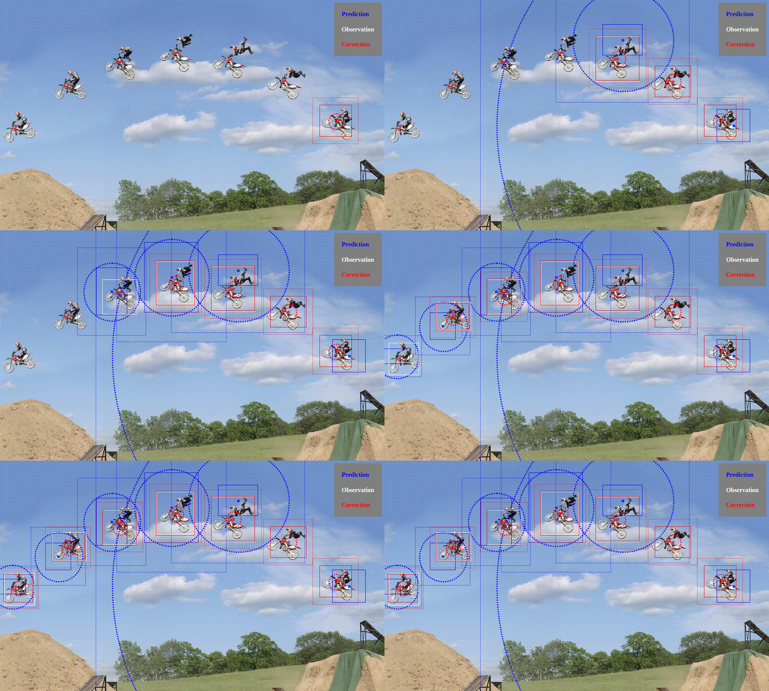 |
| Bouncing Ball | 2D constant acceleration with bounces | 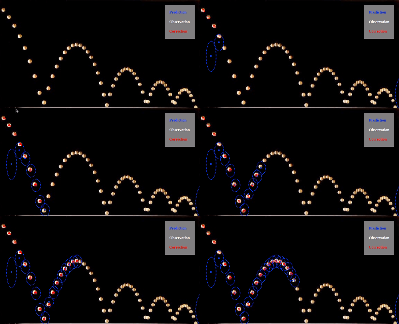 |
| Sinusoidale Extended Kalman-Filter | 1D Extended KF Sinus | 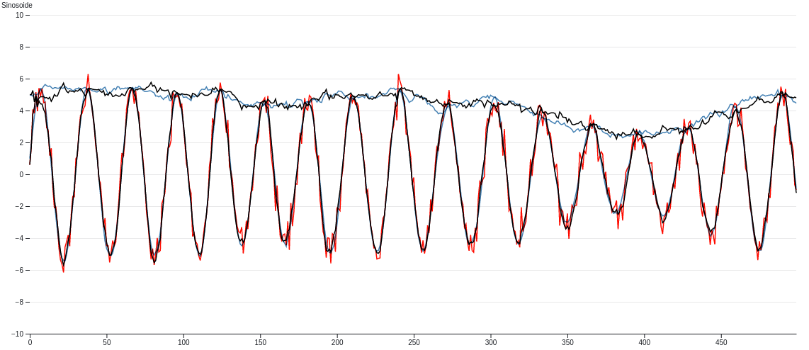 |
| Code pen GPS Data smoothing with constant speed | 2D constant speed | 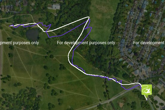 |
| Partial Observation | 1D / 2 sensor with missing values | 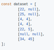 |
| Smooth 3x3 rotation matrix | 4d smoothing | 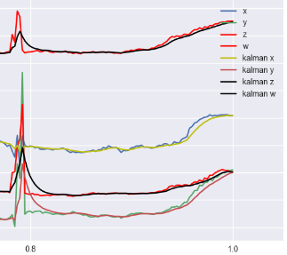 |
Open an issue to add more examples in this section explaining how you use this library !
npm install kalman-filterconst {KalmanFilter} = require('kalman-filter');Download the file kalman-filter.min.js from Releases page
Add it to your project like :
<script src="dist/kalman-filter.min.js"></script>
<script>
var {KalmanFilter} = kalmanFilter;

// ... do whatever you want with KalmanFilter

</script>const {KalmanFilter} = require('kalman-filter');
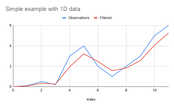
const observations = [0, 0.1, 0.5, 0.2, 3, 4, 2, 1, 2, 3, 5, 6];
// this is creating a smoothing
const kFilter = new KalmanFilter();
const res = kFilter.filterAll(observations)
// res is a list of list (for multidimensional filters)
// [
// [ 0 ],
// [ 0.06666665555510715 ],
// [ 0.3374999890620582 ],
// [ 0.25238094852592136 ],
// [ 1.9509090885288296 ],
// [ 3.2173611101031616 ],
// [ 2.4649867370240965 ],
// [ 1.5595744679428254 ],
// [ 1.831772445766021 ],
// [ 2.5537767922925685 ],
// [ 4.065625882212133 ],
// [ 5.26113483436549 ]
// ]Result is :
const {KalmanFilter} = require('kalman-filter');

const observations = [[0, 1], [0.1, 0.5], [0.2, 3], [4, 2], [1, 2]];
const kFilter = new KalmanFilter({observation: 2});
// equivalent to
// new KalmanFilter({
// 	observation: {
// 		name: 'sensor',
// 		sensorDimension: 2
// 	}
// });
const res = kFilter.filterAll(observations)const {KalmanFilter} = require('kalman-filter');
const observations = [[0, 1], [0.1, 0.5], [0.2, 3], [4, 2], [1, 2]];
const kFilter = new KalmanFilter({
observation: 2,
dynamic: 'constant-speed'
});
// equivalent to
// new KalmanFilter({
// observation: {
// name: 'sensor',
// sensorDimension: 2
// },
// dynamic: {
// name: 'constant-speed'
// },
// });
const res = kFilter.filterAll(observations)This library gives you the ability to fully configure your kalman-filter.
For advanced usage, here is the correspondance table with the matrix name of the wikipedia article
| Wikipedia article | kalman-filter js lib |
|---|---|
|
|
dynamic.transition |
|
|
observation.stateProjection |
|
|
dynamic.covariance |
|
|
observation.covariance |
|
|
dynamic.constant |
dynamic.init.covariance |
|
dynamic.init.mean |
dynamic.name is a shortcut to give you access to preconfigured dynamic models, you can also register your own shortcust see Register models shortcuts
Available default models as :
- constant-position
- constant-speed
- constant-acceleration
This will automatically configure the dynamic.transition matrix.
This is the default behavior
const {KalmanFilter} = require('kalman-filter');

const kFilter = new KalmanFilter({
	observation: {
		sensorDimension: 2,
		name: 'sensor'
	},
	dynamic: {
		name: 'constant-position',// observation.sensorDimension == dynamic.dimension
		covariance: [3, 4]// equivalent to diag([3, 4])
	}
});const {KalmanFilter} = require('kalman-filter');
const kFilter = new KalmanFilter({
observation: {
sensorDimension: 3,
name: 'sensor'
},
dynamic: {
name: 'constant-speed',// observation.sensorDimension * 2 == state.dimension
timeStep: 0.1,
covariance: [3, 3, 3, 4, 4, 4]// equivalent to diag([3, 3, 3, 4, 4, 4])
}
});const {KalmanFilter} = require('kalman-filter');
const kFilter = new KalmanFilter({
observation: {
sensorDimension: 2,
name: 'sensor'
},
dynamic: {
name: 'constant-acceleration',// observation.sensorDimension * 3 == state.dimension
timeStep: 0.1,
covariance: [3, 3, 4, 4, 5, 5]// equivalent to diag([3, 3, 4, 4, 5, 5])
}
});This is an example of how to build a constant speed model, in 3D without dynamic.name, using detailed api.
dynamic.dimensionis the size of the statedynamic.transitionis the state transition model that defines the dynamic of the systemdynamic.covarianceis the covariance matrix of the transition modeldynamic.initis used for initial state (we generally set a big covariance on it)
const {KalmanFilter} = require('kalman-filter');

const timeStep = 0.1;

const huge = 1e8;

const kFilter = new KalmanFilter({
	observation: {
		dimension: 3
	},
	dynamic: {
		init: {
			// We just use random-guessed values here that seems reasonable
			mean: [[500], [500], [500], [0], [0], [0]],
			// We init the dynamic model with a huge covariance cause we don't
			// have any idea where my modeled object before the first observation is located
			covariance: [
				[huge, 0, 0, 0, 0, 0],
				[0, huge, 0, 0, 0, 0],
				[0, 0, huge, 0, 0, 0],
				[0, 0, 0, huge, 0, 0],
				[0, 0, 0, 0, huge, 0],
				[0, 0, 0, 0, 0, huge],
			],
		},
		// Corresponds to (x, y, z, vx, vy, vz)
		dimension: 6,
		// This is a constant-speed model on 3D : [ [Id , timeStep*Id], [0, Id]]
		transition: [
			[1, 0, 0, timeStep, 0, 0],
			[0, 1, 0, 0, timeStep, 0],
			[0, 0, 1, 0, 0, timeStep],
			[0, 0, 0, 1, 0, 0],
			[0, 0, 0, 0, 1, 0],
			[0, 0, 0, 0, 0, 1]
		],
		// Diagonal covariance for independant variables
		// since timeStep = 0.1,
		// it makes sense to consider speed variance to be ~ timeStep^2 * positionVariance
		covariance: [1, 1, 1, 0.01, 0.01, 0.01]// equivalent to diag([1, 1, 1, 0.01, 0.01, 0.01])
	}
});The observation is made from 2 different sensors with identical properties (i.e. same covariances) , the input measure will be [<sensor0-dim0>, <sensor0-dim1>, <sensor1-dim0>, <sensor1-dim1>].
const {KalmanFilter} = require('kalman-filter');

const timeStep = 0.1;

const kFilter = new KalmanFilter({
	observation: {
		sensorDimension: 2,// observation.dimension == observation.sensorDimension * observation.nSensors
		nSensors: 2,
		sensorCovariance: [3, 4], // equivalent to diag([3, 4])
		name: 'sensor'
	},
	dynamic: {
		name: 'constant-speed',// observation.sensorDimension * 2 == state.dimension
		covariance: [3, 3, 4, 4]// equivalent to diag([3, 3, 4, 4])
	}
});The observation is made from 2 different sensors with different properties (i.e. different covariances), the input measure will be [<sensor0-dim0>, <sensor0-dim1>, <sensor1-dim0>, <sensor1-dim1>].
This can be achived manually by using the detailed API :
observation.dimensionis the size of the observationobservation.stateProjectionis the matrix that transforms state into observation, also called observation modelobservation.covarianceis the covariance matrix of the observation model
const {KalmanFilter} = require('kalman-filter');

const timeStep = 0.1;

const kFilter = new KalmanFilter({
	observation: {
		dimension: 4,
		stateProjection: [
			[1, 0, 0, 0],
			[0, 1, 0, 0],
			[1, 0, 0, 0],
			[0, 1, 0, 0]
		],
		covariance: [3, 4, 0.3, 0.4]
	},
	dynamic: {
		name: 'constant-speed',// observation.sensorDimension * 2 == state.dimension
		covariance: [3, 3, 4, 4]// equivalent to diag([3, 3, 4, 4])
	}
});In order to use the Kalman-Filter with a dynamic or observation model which is not strictly a General linear model, it is possible to use function in following parameters :
observation.stateProjectionobservation.covariancedynamic.transitiondynamic.covariancedynamic.constant
In this situation this function will return the value of the matrix at each step of the kalman-filter.
In this example, we create a constant-speed filter with non-uniform intervals;
const {KalmanFilter} = require('kalman-filter');

const intervals = [1,1,1,1,2,1,1,1];

const kFilter = new KalmanFilter({
	observation: {
		dimension: 2,
		/**
		* @param {State} opts.predicted
		* @param {Array.<Number>} opts.observation
		* @param {Number} opts.index
		*/
		stateProjection: function(opts){
			return [
				[1, 0, 0, 0],
				[0, 1, 0, 0]
			]
		},
		/**
		* @param {State} opts.predicted
		* @param {Array.<Number>} opts.observation
		* @param {Number} opts.index
		*/
		covariance: function(opts){
			return [
				[1, 0, 0, 0],
				[0, 1, 0, 0],
				[0, 0, 1, 0],
				[0, 0, 0, 1]
			]
		}
	},
	dynamic: {
		dimension: 4, //(x, y, vx, vy)
		/**
		* @param {State} opts.previousCorrected
		* @param {Number} opts.index
		*/
		transition: function(opts){
			const dT = intervals[opts.index];
			if(typeof(dT) !== 'number' || isNaN(dT) || dT <= 0){
				throw(new Error('dT should be positive number'))
			}
			return [
				[1, 0, dT, 0],
				[0, 1, 0, dT]
				[0, 0, 1, 0]
				[0, 0, 0, 1]
			]
		},
		/**
		* @param {State} opts.previousCorrected
		* @param {Number} opts.index
		*/
		covariance: function(opts){
			const dT = intervals[opts.index];
			if(typeof(dT) !== 'number' || isNaN(dT) || dT <= 0){
				throw(new Error('dT should be positive number'))
			}
			return [
				[1, 0, 0, 0],
				[0, 1, 0, 0],
				[0, 0, 1*dT, 0],
				[0, 0, 0, 1*dT]
			]
		}
	}
});If you want to implement an extended kalman filter
You will need to put your non-linear functions in the following parameters
observation.fndynamic.fn
See an example in Sinusoidale Extended Kalman-Filter
If you want to add a constant parameter in the dynamic model (also called control input), you can use dynamic.constant function
See an example code in demo/bouncing-ball or the result in Bouncing Ball example
const observations = [[0, 2], [0.1, 4], [0.5, 9], [0.2, 12]];

// batch kalman filter
const results = kFilter.filterAll(observations);When using online usage (only the forward step), the output of the filter method is an instance of the "State" class.
// online kalman filter
let previousCorrected = null;
const results = [];
observations.forEach(observation => {
	previousCorrected = kFilter.filter({previousCorrected, observation});
	results.push(previousCorrected.mean);
});If you want to use KalmanFilter in more advanced usage, you might want to dissociate the predict and the correct functions
// online kalman filter
let previousCorrected = null;
const results = [];
observations.forEach(observation => {
	const predicted = kFilter.predict({
		previousCorrected
	});

	 const correctedState = kFilter.correct({
		predicted,
		observation
	});

	results.push(correctedState.mean);

	// update the previousCorrected for next loop iteration
	previousCorrected = correctedState
});

console.log(results);The Forward - Backward process
// batch kalman filter
const results = kFilter.filterAll({observations, passMode: 'forward-backward'});To get more information on how to build a dynamic model, check in the code lib/dynamic/ (or lib/observation for observation models).
If you feel your model can be used by other, do not hesitate to create a Pull Request.
const {registerDynamic, KalmanFilter, registerObservation} = require('kalman-filter');

registerObservation('custom-sensor', function(opts1){
	// do your stuff
	return {
		dimension,
		stateProjection,
		covariance
	}
})

registerDynamic('custom-dynamic', function(opts2, observation){
	// do your stuff
	// here you can use the parameter of observation (like observation.dimension)
	// to build the parameters for dynamic
	return {
		dimension,
		transition,
		covariance
	}
})

const kFilter = new KalmanFilter({
	observation: {
		name: 'custom-sensor',
		// ... fields of opts1
	},
	dynamic: {
		name: 'custom-dynamic',
		// ... fields of opts2
	}
});In order to find the proper values for covariance matrix, we use following approach :
const {getCovariance, KalmanFilter} = require('kalman-filter');

// Ground truth values in the dynamic model hidden state
const groundTruthStates = [ // here this is (x, vx)
	[[0, 1.1], [1.1, 1], [2.1, 0.9], [3, 1], [4, 1.2]], // example 1
	[[8, 1.1], [9.1, 1], [10.1, 0.9], [11, 1], [12, 1.2]] // example 2
]

// Observations of this values
const measures = [ // here this is x only
	[[0.1], [1.3], [2.4], [2.6], [3.8]], // example 1
	[[8.1], [9.3], [10.4], [10.6], [11.8]] // example 2
];

const kFilter = new KalmanFilter({
	observation: {
		name: 'sensor',
		sensorDimension: 1
	},
	dynamic: {
		name: 'constant-speed'
	}
})

const dynamicCovariance = getCovariance({
	measures: groundTruthStates.map(ex =>
		return ex.slice(1)
	).reduce((a,b) => a.concat(b)),
	averages: groundTruthStates.map(ex =>
		return ex.slice(1).map((_, index) => {
			return kFilter.predict({previousCorrected: ex[index - 1]}).mean;
		})
	).reduce((a,b) => a.concat(b))
});

const observationCovariance = getCovariance({
	measures: measures.reduce((a,b) => a.concat(b)),
	averages: groundTruthStates.map((a) => a[0]).reduce((a,b) => a.concat(b))
});There are different ways to measure the performance of a model against some measures :
We use Mahalanobis distance
const observations = [[0, 2], [0.1, 4], [0.5, 9], [0.2, 12]];

// online kalman filter
let previousCorrected = null;
const results = [];

observations.forEach(observation => {
	const predicted = kFilter.predict({
		previousCorrected
	});

	const dist = predicted.mahalanobis(observation)

	previousCorrected = kFilter.correct({
		predicted,
		observation
	});

	distances.push(dist);
});

const distance = distances.reduce((d1, d2) => d1 + d2, 0);We compare the model with random generated numbers sequence.
const h = require('hasard')
const observationHasard = h.array({value: h.number({type: 'normal'}), size: 2})

const observations = observationHasard.run(200);

// online kalman filter
let previousCorrected = null;
const results = [];

observations.forEach(observation => {
	const predicted = kFilter.predict({
		previousCorrected
	});

	const dist = predicted.mahalanobis(measure)

	previousCorrected = kFilter.correct({
		predicted,
		observation
	});

	distances.push(dist);
});

const distance = distances.reduce((d1, d2) => d1 + d2, 0);Thanks to Adrien Pellissier for his hard work on this library.
For a simple 1D Kalman filter in javascript see https://github.com/wouterbulten/kalmanjs
