KAIST CS479: Machine Learning for 3D Data (Fall 2023)
Programming Assignment 3
Instructor: Minhyuk Sung (mhsung [at] kaist.ac.kr)
TA: Juil Koo (63days [at] kaist.ac.kr)
We use the same conda environment used in Assignment1. You can skip the part of creating conda environment and just install additional packages in requirements.txt following the instruction below.
conda create -n diffusion python=3.9
conda activate diffusion
conda install pytorch=1.13.0 torchvision pytorch-cuda=11.6 -c pytorch -c nvidia
conda install -c fvcore -c iopath -c conda-forge fvcore iopath
conda install pytorch3d -c pytorch3d
Lastly, install the required package within the requirements.txt
pip install -r requirements.txt
.
├── 2d_plot_diffusion_todo    (Task 1)
│   ├── ddpm_tutorial.ipynb       <--- Main code
│   ├── dataset.py                <--- Define dataset (Swiss-roll, moon, gaussians, etc.)
│   ├── network.py                <--- (TODO) Implement a noise prediction network
│   └── ddpm.py                   <--- (TODO) Define a DDPM pipeline
│
└── image_diffusion_todo (Task 2)
    ├── dataset.py                <--- Ready-to-use AFHQ dataset code
    ├── train.py                  <--- DDPM training code
    ├── sampling.py               <--- Image sampling code
    ├── ddpm.py                   <--- (TODO) Define a DDPM pipeline
    ├── module.py                 <--- Basic modules of a noise prediction network
    ├── network.py                <--- Noise prediction network of 2D images
    └── fid
        ├── measure_fid.py        <--- script measuring FID score
        └── afhq_inception.ckpt   <--- pre-trained classifier for FID
Implementation of diffusion models can be simple once you understand the theory. So, to learn the most from this assignment, it's highly recommended to check out the details in the related papers and understand the equations BEFORE you start the assignment. You can check out the resources in this order:
- [paper] Denoising Diffusion Probabilistic Models
- [paper] Denoising Diffusion Implicit Models
- [blog] Lilian Wang's "What are Diffusion Models?"
- [slide] Summary of DDPM and DDIM
More further reading materials are provided here.
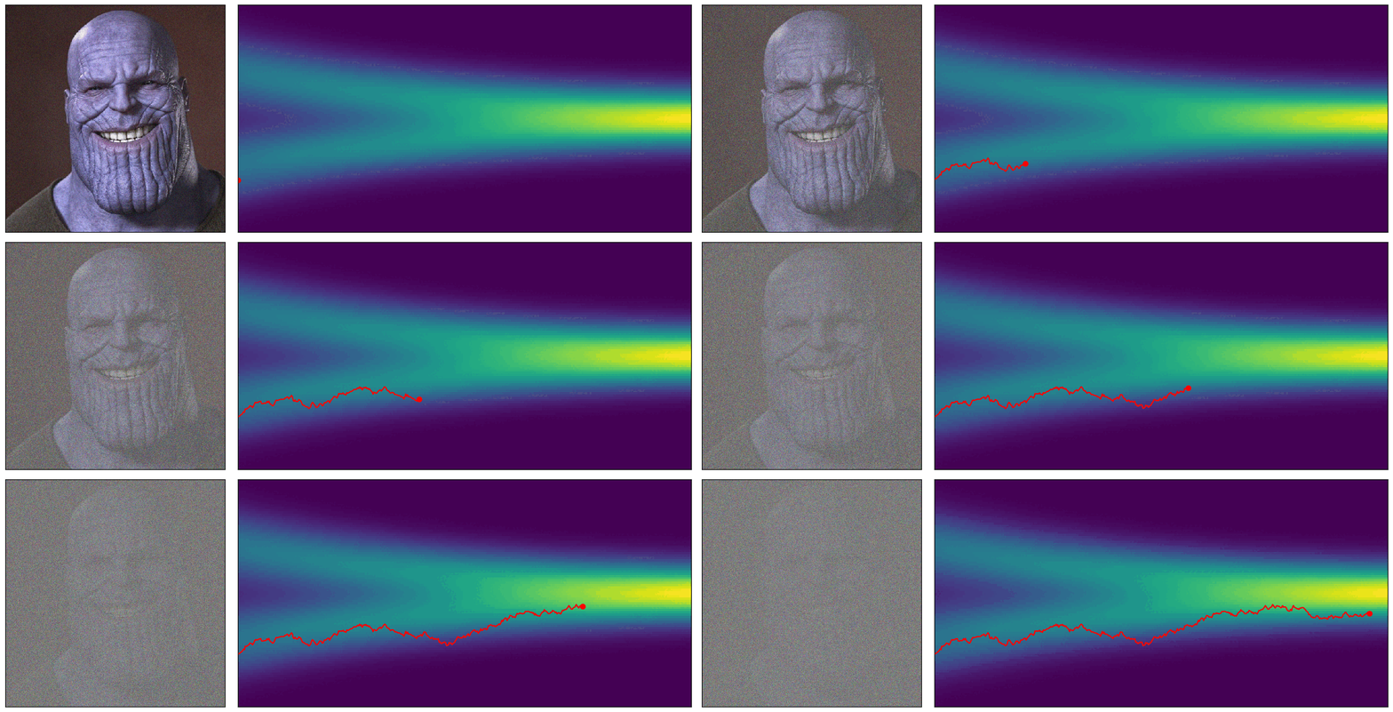
Denoising Diffusion Probabilistic Model (DDPM) is one of latent-variable generative models consisting of a Markov chain. In the Markov chain, let us define a forward process that gradually adds noise to the data sampled from a data distribution
where a variance schedule
Thanks to a nice property of a Gaussian distribution, one can directly sample
where
Refer to our slide or blog for more details.
If we can reverse the forward process, i.e. sample
where
To learn this reverse process, we set an objective function that minimizes KL divergence between
As a parameterization of DDPM, the authors set
The authors empirically found that predicting
In short, the simplified objective function of DDPM is defined as follows:
where
Refer to the original paper for more details.
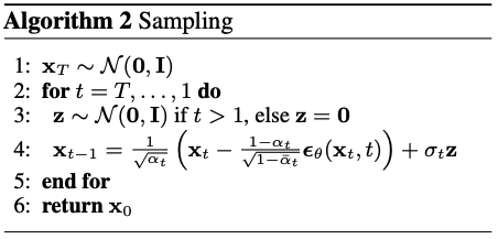
Once we train the noise prediction network
DDIM proposed a way to speed up the sampling using the same pre-trained DDPM. The reverse step of DDIM is below:
Note that
Please refer to DDIM paper for more details.
A typical diffusion pipeline is divided into three components:
In this task, we will look into each component one by one in a toy experiment and implement them sequentially.
After finishing the implementation, you will be able to train DDPM and evaluate the performance in ddpm_tutorial.ipynb under 2d_plot_todo directory.
❗️❗️❗️ You are only allowed to edit the part marked by TODO. ❗️❗️❗️
You first need to implement a noise prediction network in network.py.
The network should consist of TimeLinear layers whose feature dimensions are a sequence of [dim_in, dim_hids[0], ..., dim_hids[-1], dim_out].
Every TimeLinear layer except for the last TimeLinear layer should be followed by a ReLU activation.
Now you should construct a forward and reverse process of DDPM in ddpm.py.
q_sample() is a forward function that maps
p_sample() is a one-step reverse transition from p_sample_loop() is the full reverse process corresponding to DDPM sampling algorithm.
ddim_p_sample() and ddim_p_sample_loop() are for the reverse process of DDIM. Based on the reverse step of DDIM, implement them.
In ddpm.py, compute_loss() function should return the simplified noise matching loss in DDPM paper.
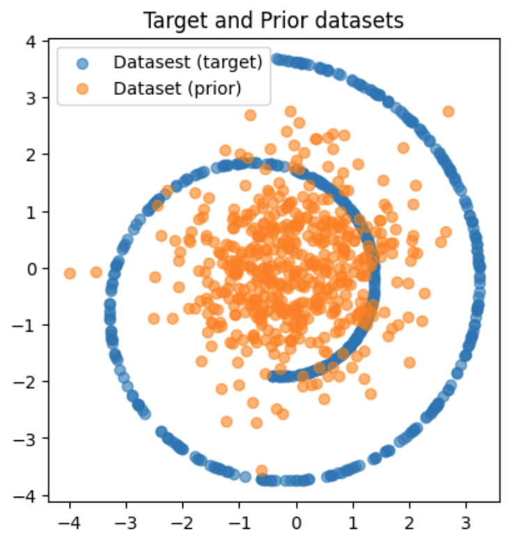
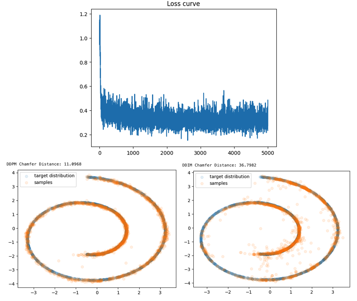
Once you finish the implementation above, open and run ddpm_tutorial.ipynb via jupyter notebook. It will automatically train a diffudion model and measure chamfer distance between 2D particles sampled by the diffusion model and 2D particles sampled from the target distribution.
Take screenshots of a loss curve as well as the chamfer distance results and visualizations of DDPM sampling and DDIM sampling.
If you successfully finish the task 1, copy 2d_plot_todo/ddpm.py into image_diffusion_todo/ddpm.py. They share the same code.
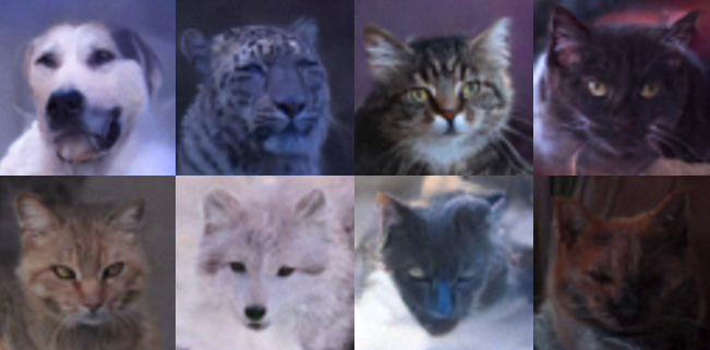
In this task, we will generate
Train a model by python train.py.
❗️❗️❗️ DO NOT modify any given hyperparameters. ❗️❗️❗️
It will sample images and save a checkpoint every args.log_interval. After training a model, sample & save images by
python sampling.py --ckpt_path ${CKPT_PATH} --save_dir ${SAVE_DIR_PATH}
We recommend starting the training as soon as possible since the training would take about half of a day. If you don't have enough time to sample images with DDPM sampling, you can use DDIM sampling which can speed up the sampling time with some sacrifice of the sample quality.
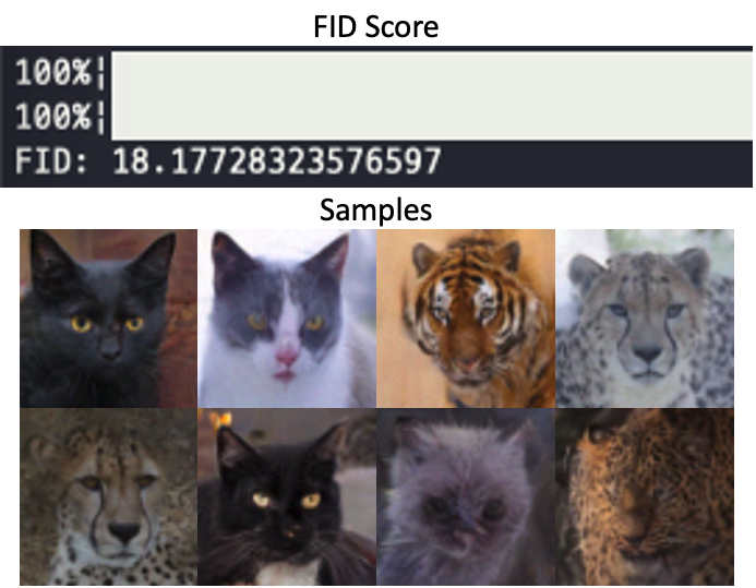
As an evaluation, measure FID score using the pre-trained classifier network we provide:
python dataset.py # to constuct eval directory.
python fid/measure_fid.py /path/to/eval/dir /path/to/sample/dir
Take a screenshot of a FID score and include at least 8 sampled images.
❗️ If you face negative FID values, it might be due to an overflow issue with the linalg.sqrtm function in the latest version of scipy. We've observed that scipy version 1.7.3 works correctly. To fix the issue, reinstall scipy to 1.7.3 version by running the command: pip install scipy=1.7.3.
Submission Item List
- Code without model checkpoints
Task 1
- Loss curve screenshot
- Chamfer distance result of DDPM sampling
- Visualization of DDPM sampling
- Chamfer distance result of DDIM sampling
- Visualization of DDIM sampling
Task 2
- FID score result
- At least 8 generated images
In a single document, write your name and student ID, and include submission items listed above. Refer to more detailed instructions written in each task section about what to submit.
Name the document {NAME}_{STUDENT_ID}.pdf and compile a ZIP file named {NAME}_{STUDENT_ID}.zip containing the following:
- The
{NAME}_{STUDENT_ID}.pdfdocument file. - All
.pyand.ipynbscript files from the Assignment3 directory. Include both the scripts you have modifed and those that already existed. - Due to file size, exclude all checkpoint files, even the provided classifier checkpoint file (
afhq_inception_v3.ckpt).
Submit the zip file on GradeScope.
You will receive a zero score if:
- you do not submit,
- your code is not executable in the Python environment we provided, or
- you modify anycode outside of the section marked with
TODOor use different hyperparameters that are supposed to be fixed as given.
Plagiarism in any form will also result in a zero score and will be reported to the university.
Your score will incur a 10% deduction for each missing item in the submission item list.
Otherwise, you will receive up to 100 points from this assignment that count toward your final grade.
- Task 1
- 50 points:
- Achieve CD lower than 20 from DDPM sampling, and
- achieve CD lower than 40 from DDIM sampling with 50 inference timesteps out of 1000 diffusion timesteps.
- 25 points: Only one of the two criteria above is successfully met.
- 0 point: otherwise.
- 50 points:
- Task 2
- 50 points: Achieve FID less than 20.
- 25 points: Achieve FID between 20 and 40.
- 0 point: otherwise.
If you are interested in this topic, we encourage you to check out the materials below.
- Denoising Diffusion Probabilistic Models
- Denoising Diffusion Implicit Models
- Diffusion Models Beat GANs on Image Synthesis
- Score-Based Generative Modeling through Stochastic Differential Equations
- What are Diffusion Models?
- Generative Modeling by Estimating Gradients of the Data Distribution
- Deep Unsupervised Learning using Nonequilibrium Thermodynamics
- Bayesian Learning via Stochastic Gradient Langevin Dynamics
