KAIST CS479: Machine Learning for 3D Data (Fall 2023)
Programming Assignment 2
Instructor: Minhyuk Sung (mhsung [at] kaist.ac.kr)
TA: Seungwoo Yoo (dreamy1534 [at] kaist.ac.kr)
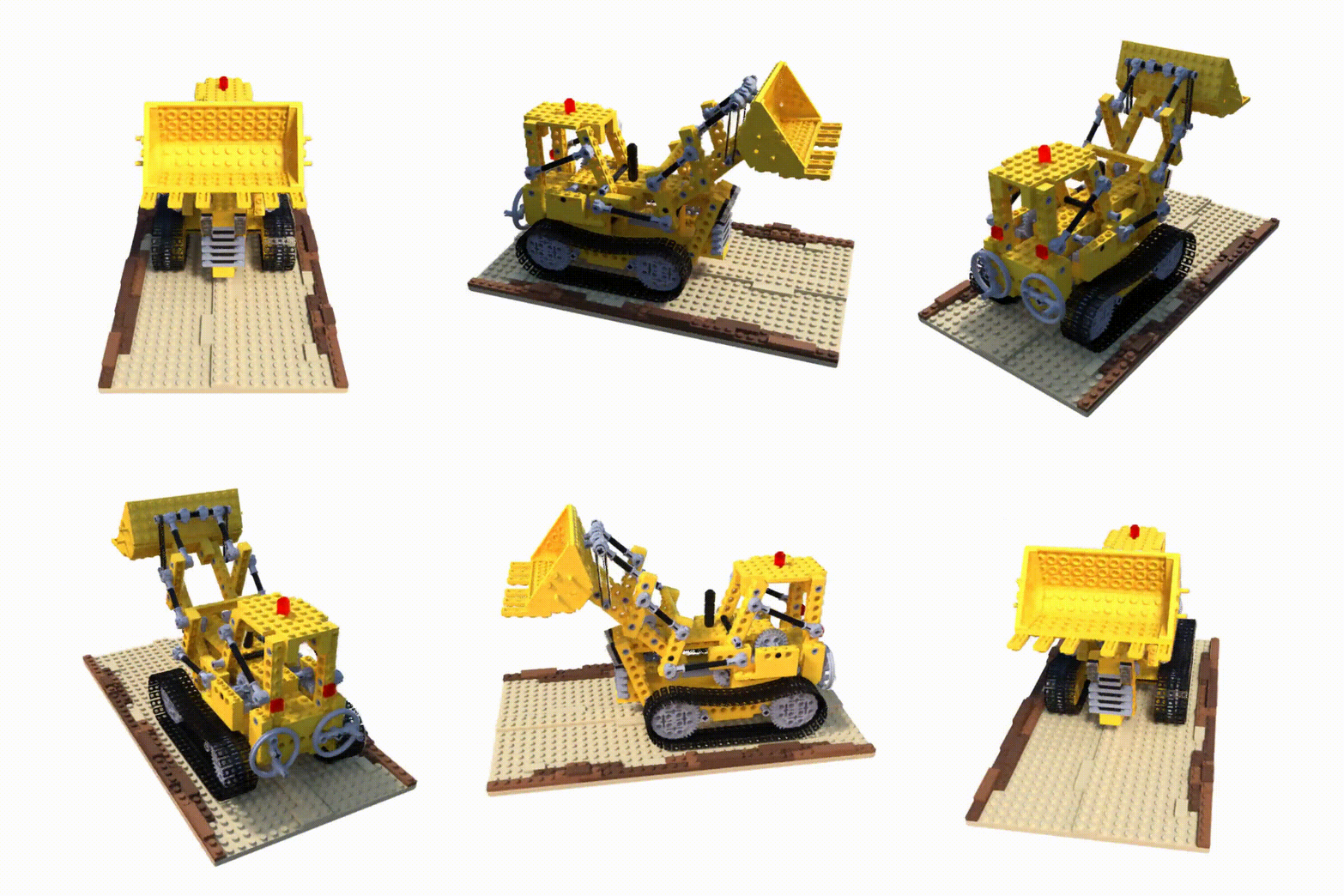
The introduction of Neural Radiance Fields (NeRF) was a massive milestone in image-based, neural rendering literature. Compared with previous works on novel view synthesis, NeRF is a simple, yet powerful idea that combines recently emerging neural implicit representations with traditional volume rendering techniques. As of today, the follow-up research aiming to scale and extend the idea to various tasks has become one of the most significant streams in the computer vision community thanks to its simplicity and versatility.
In this assignment, we will take a technical deep dive into NeRF to understand this ground-breaking approach which will help us navigate a broader landscape of the field. We strongly recommend you check out the paper, together with our brief summary, before, or while working on this assignment.
⚠️ This assignment involves training a neural network that takes approximately 2 hours. Start as early as possible.
Table of Content
We recommend creating a virtual environment using conda.
To create a conda environment, issue the following command:
conda create --name nerf-tutorial python=3.8
This should create a basic environment with Python 3.8 installed.
Next, activate the environment and install the dependencies using pip:
conda activate nerf-tutorial
pip install -r requirements.txt
The remaining dependencies are the ones related to PyTorch and they can be installed with the command:
pip install torch==1.10.1+cu113 torchvision==0.11.2+cu113 torchaudio==0.10.1 -f https://download.pytorch.org/whl/cu113/torch_stable.html
pip install torchmetrics[image]
pip install tensorboard
Register the project root directory (i.e., torch-NeRF) as an environment variable to help the Python interpreter search our files.
export PYTHONPATH=.
By default, the configuration is set for the lego scene included in the Blender dataset. Refer to the config files under config for more details. Executing the following initiates training:
python torch_nerf/runners/train.py
All by-products produced during each run, including TensorBoard logs, will be saved under an experiment directory under outputs. This is automatically done by Hydra, the library we use for managing our config files. Refer to the official documentation for examples and APIs.
We highly encourage you to try out multiple seeds as the performance of neural networks is often sensitive to the initialization.
The function init_torch that sets the random seed for PyTorch is located at torch_nerf/runners/utils.py
💡 Each run takes approximately 2 hours on a single NVIDIA RTX 3090 GPU and consumes around 10 GB of VRAM.
After training NeRF, it can be rendered using the script render.py.
To do so, provide the experiment directory created when running the training script. For instance,
python torch_nerf/runners/render.py +log_dir=outputs/2023-06-27/00-10-15 +render_test_views=False
The Boolean flag render_test_views determines whether to render the trained scene from the viewpoints held out for testing. We will come back to this when discussing quantitative evaluation.
This codebase is organized as the following directory tree. We only list the core components for brevity:
torch_nerf
│
├── configs             <- Directory containing config files
│
├── runners
│   ├── evaluate.py     <- Script for quantitative evaluation.
│   ├── render.py       <- Script for rendering (i.e., qualitative evaluation).
│   ├── train.py        <- Script for training.
│   └── utils.py        <- A collection of utilities used in the scripts above.
│
├── src
│   ├── cameras
│   │   ├── cameras.py
│   │   └── rays.py
│   │
│   ├── network
│   │   └── nerf.py
│   │
│   ├── renderer
│   │   ├── integrators
│   │   ├── ray_samplers
│   │   └── volume_renderer.py
│   │
│   ├── scene
│   │
│   ├── signal_encoder
│   │   ├── positional_encoder.py
│   │   └── signal_encoder_base.py
│   │
│   └── utils
│       ├── data
│       │   ├── blender_dataset.py
│       │   └── load_blender.py
│       │
│       └── metrics
│           └── rgb_metrics.py
│
├── requirements.txt    <- Dependency configuration file.
└── README.md           <- This file.
Download the file lego.zip from here and extract it under directory data/nerf_synthetic. The training script expects the data to be located under data/nerf_synthetic/lego.
💡
scpis a handy tool for transferring files between local and remote servers. Check this link for examples.
#! files-to-modify
$ torch_nerf/src/network/nerf.py
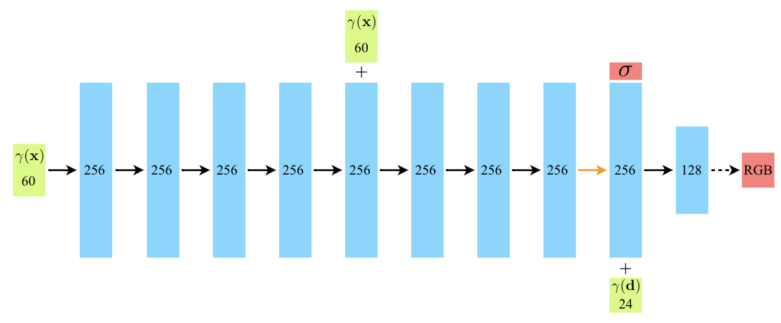
Implement the MLP displayed above. The network consists of:
- One input fully-connected layer;
- Nine fully-connected layers (including the one for skip connection);
- One output fully-connected layer.
All hidden layers are followed by ReLU activation, and the density and the RGB head at the output layer are followed by ReLU and sigmoid activations, respectively. For more details, please refer to Sec. A of the paper's supplementary material.
💡 We highly recommend you to look up the official documentation of the layers used in the network.
#! files-to-modify
$ torch_nerf/src/cameras/rays.py
$ torch_nerf/src/renderer/ray_samplers/stratified_sampler.py
This task consists of two sub-tasks:
- Implement the body of function
compute_sample_coordinatesintorch_nerf/src/cameras/rays.py. This function will be used to evaluate the coordinates of points along rays cast from image pixels. For a ray$r$ parameterized by the origin$\mathbf{o}$ and direction$\mathbf{d}$ (not necessarily a unit vector), a point on the ray can be computed by
where
- Implement the body of function
sample_along_rays_uniformintorch_nerf/src/renderer/ray_samplers/stratified_sampler.py. The function implements the stratified sampling illustrated in the following equation (Eqn 2. in the paper).
💡 Check out the helper functions
create_t_binsandmap_t_to_euclideanwhile implementing functionsample_along_rays_uniform. Also, you may findtorch.rand_likeuseful when generating random numbers for sampling.
#! files-to-modify
$ torch_nerf/src/renderer/integrators/quadrature_integrator.py
This task consists of one sub-task:
- Implement the body of function
integrate_along_rays. The function implements Eqn. 3 in the paper which defines a pixel color as a weighted sum of radiance values collected along a ray:
where
💡 The PyTorch APIs
torch.exp,torch.cumsum, andtorch.summight be useful when implementing the quadrature integration.
For qualitative evaluation, render the trained scene with the provided script.
python torch_nerf/runners/render.py +log_dir=${LOG_DIR} +render_test_views=False
This will produce a set of images rendered while orbiting around the upper hemisphere of an object.
The rendered images can be compiled into a video using the script scripts/utils/create_video.py:
python scripts/utils/create_video.py --img_dir ${RENDERED_IMG_DIR} --vid_title ${VIDEO_TITLE}
For quantitative evaluation, render the trained scene again, but from the test views.
python torch_nerf/runners/render.py +log_dir=${LOG_DIR} +render_test_views=True
This will produce 200 images (in the case of the synthetic dataset) held out during training.
After rendering images from the test view, use the script evaluate.py to compute LPIPS, PSNR, and SSIM. For instance, to evaluate the implementation for the lego scene:
python torch_nerf/runners/evaluate.py ${RENDERED_IMG_DIR} ./data/nerf_synthetic/lego/test
The metrics measured after training the network for 50k iterations on the lego scene are summarized in the following table.
| LPIPS (↓) | PSNR (↑) | SSIM (↑) |
|---|---|---|
| 0.0424 | 29.5089 | 0.9551 |
💡 For details on grading, refer to section Evaluation Criteria.
Instead of using the provided dataset, capture your surrounding environment and use the data for training. COLMAP might be useful when computing the relative camera poses.
Compile the following files as a ZIP file named {NAME}_{STUDENT_ID}.zip and submit the file via Gradescope.
- The folder
torch_nerfthat contains every source code file; - A folder named
{NAME}_{STUDENT_ID}_renderingscontaining the renderings (.pngfiles) from the test views used for computing evaluation metrics; - A text file named
{NAME}_{STUDENT_ID}.txtcontaining a comma-separated list of LPIPS, PSNR, and SSIM from quantitative evaluation; - The checkpoint file named
{NAME}_{STUDENT_ID}.pthused to produce the above metrics.
You will receive a zero score if:
- you do not submit,
- your code is not executable in the Python environment we provided, or
- you modify any code outside of the section marked with
TODO.
Plagiarism in any form will also result in a zero score and will be reported to the university.
Your score will incur a 10% deduction for each missing item in the Submission Guidelines section.
Otherwise, you will receive up to 300 points from this assignment that count toward your final grade.
| Evaluation Criterion | LPIPS (↓) | PSNR (↑) | SSIM (↑) |
|---|---|---|---|
| Success Condition (100%) | 0.06 | 28.00 | 0.90 |
| Success Condition (50%) | 0.10 | 20.00 | 0.60 |
As shown in the table above, each evaluation metric is assigned up to 100 points. In particular,
- LPIPS
- You will receive 100 points if the reported value is equal to or, smaller than the success condition (100%);
- Otherwise, you will receive 50 points if the reported value is equal to or, smaller than the success condition (50%).
- PSNR
- You will receive 100 points if the reported value is equal to or, greater than the success condition (100%);
- Otherwise, you will receive 50 points if the reported value is equal to or, greater than the success condition (50%).
- SSIM
- You will receive 100 points if the reported value is equal to or, greater than the success condition (100%);
- Otherwise, you will receive 50 points if the reported value is equal to or, greater than the success condition (50%).
If you are interested in this topic, we encourage you to check out the papers listed below.
- NeRF++: Analyzing and Improving Neural Radiance Fields (arXiv 2021)
- NeRF in the Wild: Neural Radiance Fields for Unconstrained Photo Collections (CVPR 2021)
- pixelNeRF: Neural Radiance Fields from One or Few Images (CVPR 2021)
- Mip-NeRF: A Multiscale Representation for Anti-Aliasing Neural Radiance Fields (ICCV 2021)
- BARF: Bundle-Adjusting Neural Radiance Fields (ICCV 2021)
- Nerfies: Deformable Neural Radiance Fields (ICCV 2021)
- NeuS: Learning Neural Implicit Surfaces by Volume Rendering for Multi-view Reconstruction (NeurIPS 2021)
- Volume Rendering of Neural Implicit Surfaces (NeurIPS 2021)
- Mip-NeRF 360: Unbounded Anti-Aliased Neural Radiance Fields (CVPR 2022)
- RegNeRF: Regularizing Neural Radiance Fields for View Synthesis from Sparse Inputs (CVPR 2022)
- Mega-NeRF: Scalable Construction of Large-Scale NeRFs for Virtual Fly-Throughs (CVPR 2022)
- Plenoxels: Radiance Fields without Neural Networks (CVPR 2022)
- Point-NeRF: Point-based Neural Radiance Fields (CVPR 2022)
- Instant-NGP: Instant Neural Graphics Primitives with a Multiresolution Hash Encoding (SIGGRAPH 2022)
- TensoRF: Tensorial Radiance Fields (ECCV 2022)
- MobileNeRF: Exploiting the Polygon Rasterization Pipeline for Efficient Neural Field Rendering on Mobile Architectures (CVPR 2023)
- Zip-NeRF: Anti-Aliased Grid-Based Neural Radiance Fields (ICCV 2023)

