title	subtitle	author	institute	date	lang
Julia, my new computing friend?	Julia introduction for MATLAB users	Lilian Besson and Pierre Haessig	SCEE Team, IETR, CentraleSupélec, Rennes	Thursday 14th of June, 2018	english

Note: a PDF is available here online.

« Julia, my new friend for computing and optimization? »

Intro to the Julia programming language, for MATLAB users
Date: 14th of June 2018
Who: Lilian Besson & Pierre Haessig (SCEE & AUT team @ IETR / CentraleSupélec campus Rennes)

Agenda for today [25 min]

What is Julia [3 min]
Comparison with MATLAB [3 min]
Examples of problems solved Julia [5 min]
Longer example on optimization with JuMP [10min]
Links for more information ? [2 min]

1. What is Julia ?

Developed and popular from the last 7 years
Open-source and free programming language (MIT license)
Interpreted and compiled, very efficient
But easy syntax, dynamic typing, inline documentation etc
Multi-platform (Windows, Mac OS X, GNU/Linux etc)
MATLAB-like imperative style
MATLAB-like syntax for linear algebra etc
Designed to be simple to learn and use
Easy to run your code in parallel (multi-core & cluster)
Used worldwide: research, data science, finance etc…

Ressources

Website:
- JuliaLang.org for the language
- & Pkg.JuliaLang.org for packages
Documentation : docs.JuliaLang.org

Comparison with MATLAB

	Julia 😃	MATLAB 😢
Cost	Free ✌️	Hundreds of euros / year
License	Open-source	1 year user license (no longer after your PhD!)
Comes from	A non-profit foundation, and the community	MathWorks company
Scope	Mainly numeric	Numeric only
Performances	Very good performance	Faster than Python, slower than Julia
Packaging	`Pkg` manager included. Based on `git` + GitHub, very easy to use	Toolboxes already included but 💰 have to pay if you wat more!
Editor/IDE	Jupyter is recommended (Juno is also good)	Good IDE already included
Parallel computations	Very easy, low overhead cost	Possible, high overhead
Usage	Generic, worldwide 🌎	Research in academia and industry
Fame	Young but starts to be known	Old and known, in decline
Support?	Community$^1$ (StackOverflow, mailing lists etc).	By MathWorks
Documentation	OK and growing, inline/online	OK, inline/online

Note$^1$: JuliaPro offer paid licenses, if professional support is needed.

How to install Julia ⬇️

You can try online for free on JuliaBox.com
On Linux, Mac OS or Windows:
- You can use the default installer 📦 from the website julialang.org/downloads
Takes about 4 minutes... and it's free !

You also need Python 3 to use Jupyter ✨, I suggest to use Anaconda.com/download if you don't have Python yet.

Select the binary of your platform 📦
Run the binary 🏃 !
Wait 🕜…
Done 👌 ! Test with julia in a terminal

Different tools to use Julia

Use julia for the command line for short experiments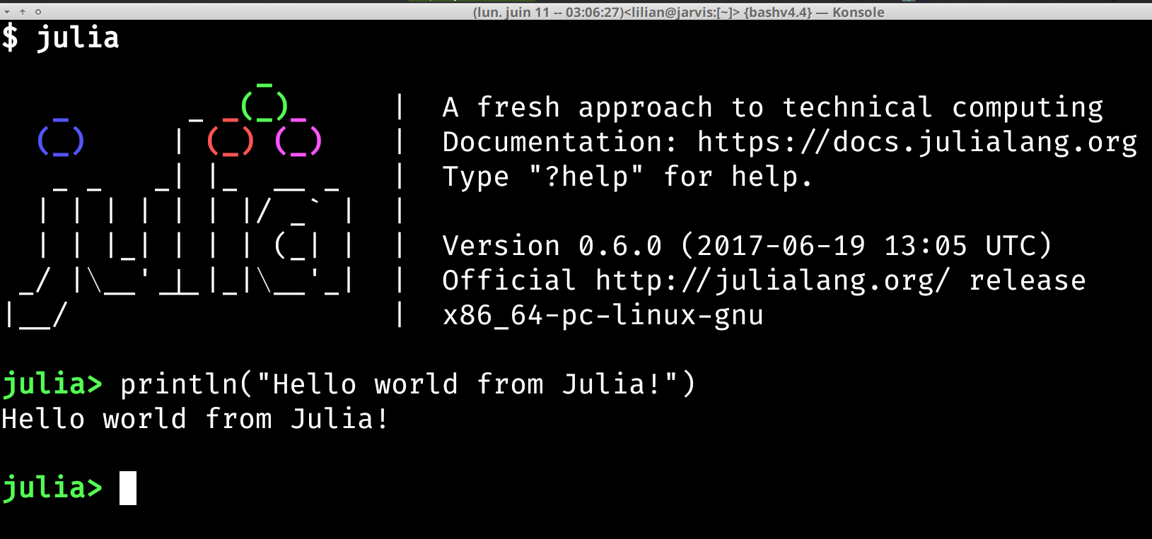
Use the Juno IDE to edit large projects

Demo time ⌚ !

Use Jupyter notebooks to write or share your experiments (examples: github.com/Naereen/notebooks)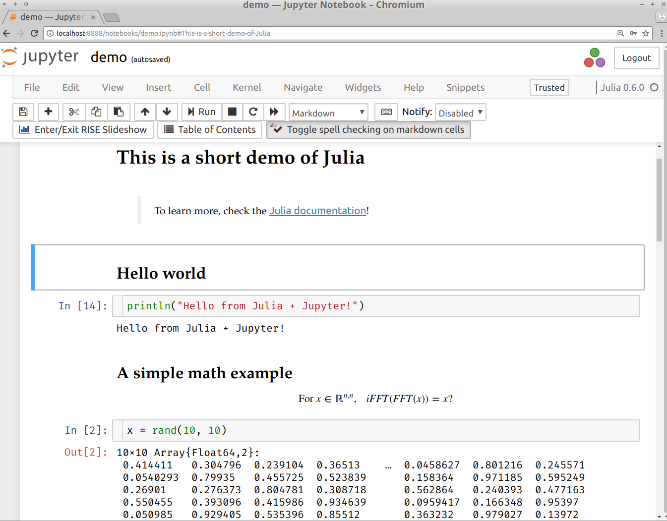

Demo time ⌚ !

📦 How to install modules in Julia ?

Installing is easy !

julia> Pkd.add("IJulia")  # installs IJulia

Updating also!

julia> Pkg.update()

🔍 How to find the module you need ?

First… ask your colleagues 😄 !
Complete list on pkg.JuliaLang.org

📦 Overview of famous Julia modules

Plotting:
- Winston.jl for easy plotting like MATLAB
- PyPlot.jl interface to Matplotlib (Python)
The JuliaDiffEq collection for differential equations
The JuliaOpt collection for optimization
The JuliaStats collection for statistics
And many more!

Find more specific packages on GitHub.com/svaksha/Julia.jl/

Many packages, and a quickly growing community

Julia is still in development, in version v0.6 but version 1.0 is planned soon!

2. Main differences in syntax between Julia and MATLAB

Ref: cheatsheets.quantecon.org

	Julia	MATLAB
File ext.	`.jl`	`.m`
Comment	`# blabla...`	`% blabla...`
Indexing	`a[1]` to `a[end]`	`a(1)` to `a(end)`
Slicing	`a[1:100]` (view)	`a(1:100)` (:warning: copy)
Operations	Linear algebra by default	Linear algebra by default
Block	Use `end` to close all blocks	Use `endif` `endfor` etc
Help	`?func`	`help func`
And	`a & b`	`a && b`
Or	`a	b`
Datatype	`Array` of any type	multi-dim doubles array
Array	`[1 2; 3 4]`	`[1 2; 3 4]`
Size	`size(a)`	`size(a)`
Nb Dim	`ndims(a)`	`ndims(a)`
Last	`a[end]`	`a(end)`
Tranpose	`a.'`	`a.'`
Conj. transpose	`a'`	`a'`
Matrix x	`a * b`	`a * b`
Element-wise x	`a .* b`	`a .* b`
Element-wise /	`a ./ b`	`a ./ b`
Element-wise ^	`a ^ 3`	`a .^ 3`
Zeros	`zeros(2, 3, 5)`	`zeros(2, 3, 5)`
Ones	`ones(2, 3, 5)`	`ones(2, 3, 5)`
Identity	`eye(10)`	`eye(10)`
Range	`range(0, 100, 2)` or `1:2:100`	`1:2:100`
Maximum	`max(a)`	`max(max(a))` ?
Random matrix	`rand(3, 4)`	`rand(3, 4)`
L2 Norm	`norm(v)`	`norm(v)`
Inverse	`inv(a)`	`inv(a)`
Solve syst.	`a \ b`	`a \ b`
Eigen vals	`V, D = eig(a)`	`[V,D]=eig(a)`
FFT/IFFT	`fft(a)`, `ifft(a)`	`fft(a)`,`ifft(a)`

Very close to MATLAB for linear algebra!

3. Scientific problems solved with Julia

Just to give examples of syntax and modules

1D numerical integration and plot
Solving a $2^{\text{nd}}$ order Ordinary Differential Equation

3.1. 1D numerical integration and plot

Exercise : evaluate and plot this function on [-1, 1] : $$\mathrm{Ei}(x) := \int_{-x}^{\infty} \frac{\mathrm{e}^u}{u} ;\mathrm{d}u$$

How to?

Use packages and everything is easy!

QuadGK.jl for integration
Winston.jl for 2D plotting

using QuadGK

function Ei(x, minfloat=1e-3, maxfloat=100)
    f = t -> exp(-t) / t  # inline function
    if x > 0
        return quadgk(f, -x, -minfloat)[1]
             + quadgk(f, minfloat, maxfloat)[1]
    else
        return quadgk(f, -x, maxfloat)[1]
    end
end

X = linspace(-1, 1, 1000)   # 1000 points
Y = [ Ei(x) for x in X ]

using Winston
plot(X, Y)
title("The function Ei(x)")
xlabel("x"); ylabel("y")
savefig("figures/Ei_integral.png")

3.2. Solving a $2^{\text{nd}}$ order ODE

Goal : solve and plot the differential equation of a pendulum: $$\theta''(t) + b ,\theta'(t) + c ,\sin(\theta(t)) = 0$$ For $b = 1/4$, $c = 5$, $\theta(0) = \pi - 0.1$, $\theta'(0)=0$, $t\in[0,10]$

How to?

Use packages!

DifferentialEquations.jl function for ODE integration
Winston.jl for 2D plotting

using DifferentialEquations

b, c = 0.25, 5.0

# macro magic!
pend2 = @ode_def Pendulum begin
  dθ = ω  # ← yes, this is UTF8, θ and ω in text
  dω = (-b * ω) - (c * sin(θ))
end

prob = ODEProblem(pend, y0, (0.0, 10.0))
sol = solve(prob)         # ↑ solve on interval [0,10]
t, y = sol.t, hcat(sol.u...)'

using Winston
plot(t, y[:, 1], t, y[:, 2])
title("2D Differential Equation")
savefig("figures/Pendulum_solution.png")

Examples

Iterative computation: signal filtering
Optimization: robust regression on RADAR data

Ex. 1: Iterative computation

Objective:

show the efficiency of Julia's Just-in-Time (JIT) compilation
but also its fragility...

Iterative computation: signal filtering

The classical saying:

« Vectorized code often runs much faster than the corresponding code containing loops. » (cf. MATLAB doc)

does not hold for Julia, because of its Just-in-Time compiler.

Example of a computation that cannot be vectorized

Smoothing of a signal ${u_k}_{k\in\mathbb{N}}$:

$$ y_k = ay_{k-1} + (1-a) u_k, k\in\mathbb{N}^+ $$

Parameter $a$ tunes the smoothing (none: $a=0$, strong $a\to1^-$).

💥 Iteration (for loop) cannot be avoided.

NB : Matlab also has JIT but it may not work well in all cases.

Signal filtering in Julia 👌

function smooth(u, a)
    y = zeros(u)

    y[1] = (1-a)*u[1]
    for k=2:length(u)  # this loop is NOT slow!
        y[k] = a*y[k-1] + (1-a)*u[k]
    end

    return y
end

Performance of the signal filter

Implementation	Time for $10 ,\mathrm{Mpts}$	notes
Julia	$50-70,\mathrm{ms}$	Fast! Easy! 👌
Octave native	$88000,\mathrm{ms}$	slow!! 🐌
Python native	$4400,\mathrm{ms}$	slow! 🐌
SciPy's `lfilter`	$70,\mathrm{ms}$	many lines of C
Python + `@numba.jit`	$50,\mathrm{ms}$	since $2012$

@numba.jit # <- factor ×100 speed-up!
def smooth_jit(u, a):
    y = np.zeros_like(u)
    y[0] = (1-a)*u[0]
    for k in range(1, len(u)):
        y[k] = a*y[k-1] + (1-a)*u[k]
    return y

Conclusion on the performance

For this simple iterative computation:

Julia performs very well, much better than native Python
but it's possible to get the same with fresh Python tools (Numba)
more realistic examples are needed

Fragility of Julia's JIT Compilation 💥

The efficiency of the compiled code relies on type inference.

function smooth1(u, a)
    y = 0
    for k=1:length(u)
        y = a*y + (1-a)*u[k]
    end
    return y
end

function smooth2(u, a)
    y = 0.0   # <- difference is here!
    for k=1:length(u)
        y = a*y + (1-a)*u[k]
    end
    return y
end

An order of magnitude difference 🐌vs🏃‍♂️

julia> @time smooth1(u, 0.9);
  0.212018 seconds (30.00 M allocations: 457.764 MiB ...)

julia> @time smooth2(u, 0.9);
  0.024883 seconds (5 allocations: 176 bytes)

Fortunately, Julia gives a good diagnosis tool 🛠️

julia> @code_warntype smooth1(u, 0.9);
...  # ↓ we spot a detail
y::Union{Float64, Int64}
...

y is either Float64 or Int64 when it should be just Float64.

Cause: initialization y=0 vs. y=0.0!

Ex. 2: Optimization in Julia

Objective: demonstrate JuMP, a Modeling Language for Optimization in Julia.

Some research groups migrate to Julia just for this package!

Cf. JuMP.ReadTheDocs.io for documentation!

Optimization problem

Example problem: identifying the sea clutter in Weather Radar data.

is a robust regression problem
- $\hookrightarrow$ is an optimization problem!

References

An « IETR-colored » example, inspired by:

Radar data+photo: P.-J. Trombe et al., « Weather radars – the new eyes for offshore wind farms?,» Wind Energy, 2014.
Regression methods: S. Boyd and L. Vandenberghe, Convex Optimization. Cambridge University Press, 2004. (Example 6.2).

Weather radar: the problem of sea clutter

Given $n$ data points $(x_i, y_i)$, fit a linear trend:

$$\hat{y} = a.x + b$$

An optimization problem with two parameters: $a$ (slope), $b$ (intercept)

Regression as an optimization problem

The parameters for the trend $(a,b)$ should minimize a criterion $J$ which penalizes the residuals $r_i = y_i - \hat{y} = y_i - a.x + b$:

$$J(a,b) = \sum_i \phi(r_i)$$

where $\phi$ is the penaly function, to be chosen:

$\phi(r) = r^2$: quadratic deviation $\rightarrow$ least squares regression
$\phi(r) = \lvert r \rvert$: absolute value deviation
$\phi(r) = h(r)$: Huber loss
...

🔧 Choice of penalty function

The choice of the loss function influences:

the optimization result (fit quality)
- e.g., in the presence of outliers
the properties of optimization problem: convexity, smoothness

Properties of each function

quadratic: convex, smooth, heavy weight for strong deviations
absolute value: convex, not smooth
Huber: a mix of the two

🛠️ How to solve the regression problem?

Option 1: a big bag of tools

A specific package for each type of regression:

« least square toolbox » ($\rightarrow$ MultivariateStats.jl)
« least absolute value toolbox » ($\rightarrow$ quantile regression)
« Huber toolbox » (i.e., robust regression $\rightarrow$ ???)
...

Option 2: the « One Tool »

$\Longrightarrow$ a Modeling Language for Optimization

more freedom to explore variants of the problem

Modeling Languages for Optimization

Purpose: make it easy to specify and solve optimization problems without expert knowledge.

JuMP: optimization modeling in Julia

The JuMP package offers a domain-specific modeling language for mathematical optimization.

JuMP interfaces with many optimization solvers: open-source (Ipopt, GLPK, Clp, ECOS...) and commercial (CPLEX, Gurobi, MOSEK...).

Other Modeling Languages for Optimization:
- Standalone software: AMPL, GAMS
- Matlab: YALMIP (previous seminar), CVX
- Python: Pyomo, PuLP, CVXPy

Claim: JuMP is fast, thanks to Julia's metaprogramming capabilities (generation of Julia code within Julia code).

📈 Regression with JuMP — common part

Given x and y the $300$ data points:

m = Model(solver = ECOSSolver())

@variable(m, a)
@variable(m, b)

res = a*x .- y + b

res (« residuals ») is an Array of $300$ elements of type JuMP.GenericAffExpr{Float64,JuMP.Variable}, i.e., a semi-symbolic affine expression.

Now, we need to specify the penalty on those residuals.

Regression choice: least squares regression

$$\min \sum_i r_i^2$$

Reformulated as a Second-Order Cone Program (SOCP):

$$\min j, \quad \text{such that} ; \lVert r \rVert_2 \leq j$$

@variable(m, j)
@constraint(m, norm(res) <= j)
@objective(m, Min, j)

(SOCP problem $\Longrightarrow$ ECOS solver)

Regression choice: least absolute deviation

$$\min \sum_i \lvert r_i \rvert $$

Reformulated as a Linear Program (LP)

$$\min \sum_i t_i, \quad \text{such that} ; -t_i \leq r_i \leq t_i$$

@variable(m, t[1:n])
@constraint(m, res .<= t)
@constraint(m, res .>= -t)
@objective(m, Min, sum(t))

Solve! ⚙️

julia> solve(m)
[solver blabla... ⏳ ]
:Optimal  # hopefully

julia> getvalue(a), getvalue(b)
(-1.094, 127.52)  # for least squares

Observations:

least abs. val., Huber ✅
least squares ❎

JuMP: summary 📜

A modeling language for optimization, within Julia:

gives access to all classical optimization solvers
very fast (claim)
gives freedom to explore many variations of an optimization problem (fast prototyping)

🗒️ More on optimization with Julia:

JuliaOpt: host organization of JuMP
Optim.jl: implementation of classics in Julia (e.g., Nelder-Mead)
JuliaDiff: Automatic Differentiation to compute gradients, thanks to Julia's strong capability for code introspection

Conclusion

Sum-up

I hope you got a good introduction to Julia 👌
It's not hard to migrate from MATLAB to Julia
Good start: docs.JuliaLang.org/en/stable/manual/getting-started
Julia is fast!
Free and open source!
Can be very efficient for some applications!

Thanks for joining 👏 !

Your mission, if you accept it... 💥

👶 Padawan level: Train yourself a little bit on Julia $\hookrightarrow$ JuliaBox.com ? Or install it on your laptop! And ead introduction in the Julia manual!
👩‍🎓 Jedi level: Try to solve a numerical system, from your research or teaching, in Julia instead of MATLAB
⚔️ Master level: From now on, try to use open-source & free tools for your research (Julia, Python and others)… 🤑

pierre-haessig/julia-presentation-ietr2018

« Julia, my new friend for computing and optimization? »

Agenda for today [25 min]

1. What is Julia ?

Ressources

Comparison with MATLAB

How to install Julia ⬇️

Different tools to use Julia

📦 How to install modules in Julia ?

🔍 How to find the module you need ?

📦 Overview of famous Julia modules

Many packages, and a quickly growing community

2. Main differences in syntax between Julia and MATLAB

3. Scientific problems solved with Julia

3.1. 1D numerical integration and plot

How to?

3.2. Solving a $2^{\text{nd}}$ order ODE

How to?

Examples

Ex. 1: Iterative computation

Iterative computation: signal filtering

Example of a computation that cannot be vectorized

Signal filtering in Julia 👌

Performance of the signal filter

Conclusion on the performance

Fragility of Julia's JIT Compilation 💥

An order of magnitude difference 🐌vs🏃‍♂️

Fortunately, Julia gives a good diagnosis tool 🛠️

Ex. 2: Optimization in Julia

Optimization problem

Weather radar: the problem of sea clutter

Regression as an optimization problem

🔧 Choice of penalty function

Properties of each function

🛠️ How to solve the regression problem?

Option 1: a big bag of tools

Option 2: the « One Tool »

Modeling Languages for Optimization

JuMP: optimization modeling in Julia

📈 Regression with JuMP — common part

Regression choice: least squares regression

Regression choice: least absolute deviation

Solve! ⚙️

JuMP: summary 📜

Conclusion

Sum-up

Your mission, if you accept it... 💥