by Diego Takahashi1 and Vanderlei C. Oliveira Jr.1
This paper has been submitted for publication in Geoscientific Model Development (GMD).
A considerable amount of literature has been published on the magnetic modelling of uniformly magnetized ellipsoids since the second half of the nineteenth century. Ellipsoids have flexibility to represent a wide range of geometrical forms, are the only known bodies which can be uniformly magnetized in the presence of a uniform inducing field and are the only finite bodies for which the self-demagnetization can be treated analytically. This property makes ellipsoids particularly useful for modelling compact orebodies having high susceptibility. In this case, neglecting the self-demagnetization may strongly mislead the interpretation of these bodies by using magnetic methods. A number of previous studies consider that the self-demagnetization can be neglected for the case in which the geological body has an isotropic susceptibility lower than or equal to 0.1 SI. This limiting value, however, seems to be determined empirically and there has been no discussion about how this value was determined. In addition, the geoscientific community lacks an easy-to-use tool to simulate the magnetic field produced by uniformly magnetized ellipsoids. Here, we present an integrated review of the magnetic modelling of arbitrarily oriented triaxial, prolate and oblate ellipsoids. Our review includes ellipsoids with both induced and remanent magnetization, as well as with isotropic or anisotropic susceptibility. We also discuss the ambiguity between confocal ellipsoids with the same magnetic moment and propose a way of determining the isotropic susceptibility above which the self-demagnetization must be taken into consideration. Tests with synthetic data validate our approach. Finally, we provide a set of routines to model the magnetic field produced by ellipsoids. The routines are written in Python language as part of the Fatiando a Terra, which is an open-source library for modelling and inversion in geophysics.
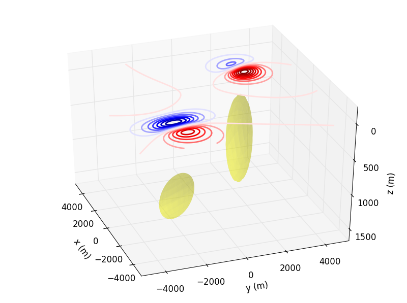
Figure 1: Total-field anomaly produced by two triaxial ellipsoids. Red lines indicate high values and blue lines indicate low values.
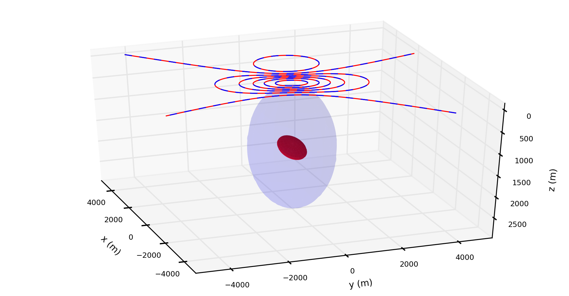
Figure 2: Total-field anomalies produced by two confocal triaxial ellipsoids. The solid red lines represent the total-field anomaly produced by the red ellipsoid. The dashed blue lines represent the total-field anomaly produced by the blue ellipsoid.
You can download a copy of all the files in this repository by cloning the git repository:
git clone https://github.com/pinga-lab/magnetic-ellipsoid.git
All source code used to generate the results and figures in the paper are in
the code folder. The sources for the manuscript text and figures are in manuscript.
See the README.md files in each directory for a full description.
The calculations and figure generation are all run inside Jupyter notebooks. You can view a static (non-executable) version of the notebooks in the nbviewer webservice:
http://nbviewer.jupyter.org/github/pinga-lab/magnetic-ellipsoid
See sections below for instructions on executing the code.
You'll need a working Python 2.7 environment with all the standard scientific packages installed (numpy, scipy, matplotlib, etc). The easiest (and recommended) way to get this is to download and install the Anaconda Python distribution. Make sure you get the Python 2.7 version.
Use conda package manager (included in Anaconda) to create a
virtual environment with
all the required packages installed.
Run the following command in this folder (where environment.yml
is located):
conda env create
To activate the conda environment, run
source activate ellipsoids
or, if you're on Windows,
activate ellipsoids
This will enable the environment for your current terminal session. After running the code, deactivate the environment with the following commands:
source deactivate
or, if you're on Windows,
deactivate
Windows users: We recommend having a bash shell and the make installed
to run the code, produce the results and check the code. You may download the
Git for Windows and the
Software Carpentry Windows Installer.
To execute the code in the Jupyter notebooks, you must first start the notebook server by going into the repository folder and running:
jupyter notebook
Make sure you have the conda environment enabled first.
This will start the server and open your default web browser to the Jupyter
interface. In the page, go into the code folder and select the
notebook that you wish to view/run.
The notebook is divided into cells (some have text while other have code).
Each cell can be executed using Shift + Enter.
Executing text cells does nothing while executing code cells runs the code
and produces it's output.
To execute the whole notebook, run all cells in order or use "Cell -> Run All"
from the menu bar.
Archived version at Zenodo
You can also find an archived version of the code at:
All source code is made available under a BSD 3-clause license. You can freely
use and modify the code, without warranty, so long as you provide attribution
to the authors. See LICENSE.md for the full license text.
The manuscript text is not open source. The authors reserve the rights to the article content, which is currently submitted for publication in Geoscientific Model Development (GMD).

