The pyproject.toml document the required dependencies. It's suggested to use the Poetry packaging tool. In this case, just issue the poetry install command to set up a virtual environment with all the necessary dependencies.
After the development environment has set up, run the notebooks in the following order to reproduce the results.
- plot_heatmaps.ipynb
- this will reproduce the heatmaps [Figure 6] from the data description paper,
- do the inverse-transformed plots, and
- some related plots for the paper
- generate_grid.ipnyb
- this will locate the observation area within Japan and generate the grid
These two notebooks contain the main work. The detect_homes.ipynb, validate_home_detection.ipynb, calculate_grid_complexity.ipynb, and the src/plot_grid.ipynb are optional steps to reproduce the figure in the technical validation section of the paper.
- Upscale heatmap as a template
- merges the neighboring cells while summing the activity in the four cells resulting lower resolution template heatmaps
- Locate upscaled observation area
- plots the land area of the selected six prefectures proportionally to the upscaled heatmap (grid) and applies template matching
- Helsinki
- the Helsinki notebook processes the data for different grid sizes in one run
- London
rxandryparameters are for the grid size, use either 500, 1000, 2000, or 4000
- Toronto
- it is the same notebook as for London, because the dataset is the same
- enable the Toronto parameter block
- Dallas--Fort Worth
RESparameter is for the H3 resolution, vales between 6 and 10 were applied
A user is considered k-identifiable if the most frequently visited k location are distinguishable 1. The top four location have been determined for every user, then the grid cell were upscaled to 1, 2, 4, 8, and 16 km.
The following table compares the top-four-location identifiable users by upscaled grids. The relevant notebook is here.
| distinguishable cells | 1 km x 1 km | 2 km x 2 km | 4 km x 4 km | 8 km x 8 km | 16 km x 16 km |
|---|---|---|---|---|---|
| 4 | 35469 | 12882 | 5090 | 1810 | 470 |
| 3 | 48228 | 42323 | 28457 | 16752 | 7438 |
| 2 | 15582 | 38548 | 50987 | 52608 | 44939 |
| 1 | 721 | 6247 | 15466 | 28830 | 47153 |
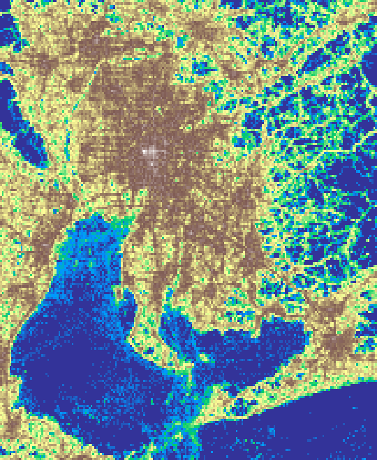
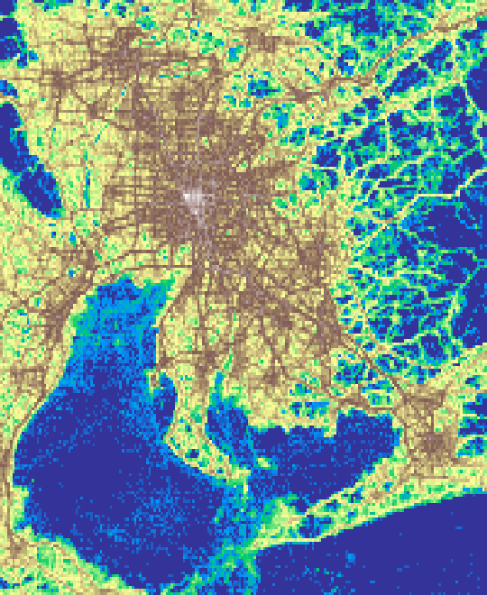
The results are included to be available without executing the code. Most notably, the reproduced grid (in EPSG:2449 projection).
The spatial distribution of the activity (first) and the number of unique users (second) per cell using the reproduced grid.
- Mobility data: YJMob100K
- details about how to prepare it
- OpenStreetMap data
- Copyrighted by OpenStreetMap contributors. It is available under the Open Database License (ODbL).
- Administrative data is from OpenStreetMap
- downloaded from OSM-Boundaries
- prefectures (admin level 4), then filtered manually
- municipalities (admin level 7), then filtered manually
- wards (admin level 8), then filtered to Nagoya
- downloaded from OSM-Boundaries
- Coastline is downloaded from https://osmdata.openstreetmap.de/data/land-polygons.html
- the islands of Japan was extracted using the prefecture boundaries
- Census data
- The Population Census 2020, Population, Households, Sex, Age and Marital status, Table 1-1 was downloaded from the Portal Site of Official Statistics of Japan website (https://www.e-stat.go.jp/)
- The code is licensed under BSD-3-Clause
- The documentation and figures are CC BY 4.0
- The shape files are from OpenStreetMap and licensed under the Open Data Commons Open Database License (ODbL)
- The census data was downloaded from the Portal Site of Official Statistics of Japan website (https://www.e-stat.go.jp/)
Footnotes
-
Hui Zang and Jean Bolot. 2011. Anonymization of location data does not work: a large-scale measurement study. In Proceedings of the 17th annual international conference on Mobile computing and networking (MobiCom '11). Association for Computing Machinery, New York, NY, USA, 145–156. https://doi.org/10.1145/2030613.2030630 ↩

