This package may be used to plot exon and splice junction coverage
across a large cohort of RNA-seq samples. The plotting approach is based
on the idea of transposing expression heatmaps on splicing diagrams. The
plots are generated using the ggplot2 and ggbio packages.
## load annotations packages
library("TxDb.Hsapiens.UCSC.hg19.knownGene")
library("BSgenome.Hsapiens.UCSC.hg19")

## load current package
devtools::load_all()
First we must construct a concomp object from a GRangesList object
with exon and junction boundaries and corresponding coverage values. For
illustration purposes, we use a previously constructed GRanges object,
klk12_lusc_gr, containing annotation information for the KLK12 gene
locus along with coverage for 177 lung squamous cell carcinoma samples.
data("klk12_lusc_gr")
The exon and junction boundaries, and the corresponding kind label are given by:
ranges(klk12_lusc_gr)

## IRanges object with 25 ranges and 0 metadata columns:
##             start       end     width
##         <integer> <integer> <integer>
##   33127  51532348  51532468       121
##   33128  51532468  51532598       131
##   33129  51532469  51532597       129
##   33130  51532598  51532713       116
##   33131  51532713  51534044      1332
##     ...       ...       ...       ...
##   33147  51537896  51538051       156
##   33148  51537896  51538062       167
##   33149  51537897  51538040       144
##   33150  51538051  51538061        11
##   33151  51538062  51538261       200

mcols(klk12_lusc_gr)$kind

##  [1] "e" "j" "e" "e" "j" "e" "j" "j" "j" "e" "e" "j" "e" "j" "j" "j" "j"
## [18] "e" "e" "e" "j" "j" "e" "e" "e"
In addition to kind, the klk12_lusc_gr metadata columns also include
the gene name (gIdx), gene boundaries (gStart, gStop), and
coverage values for the 177 samples.
mcols(klk12_lusc_gr)[1:5, 1:6]

## DataFrame with 5 rows and 6 columns
##          gIdx    gStart     gStop        kind        s1        s2
##   <character> <numeric> <numeric> <character> <numeric> <numeric>
## 1    gene9317  51532348  51538261           e   2.60331   5.32231
## 2    gene9317  51532348  51538261           j   0.00000   0.00000
## 3    gene9317  51532348  51538261           e   2.59690  10.37210
## 4    gene9317  51532348  51538261           e   2.15517   7.28448
## 5    gene9317  51532348  51538261           j   0.00000   7.00000
To construct the concomp (connected component) object for analysis, we
first convert the GRanges object into a GRangesList object of length
2, corresponding to exon and junction information.
klk12_gl <- split(klk12_lusc_gr, mcols(klk12_lusc_gr)$kind)
klk12_cc <- concomp(klk12_gl)
We first demonstrate the default and basic SpliceGraHM (Splice Graph Heat Map) plotting procedure.
splicegrahm(klk12_cc)
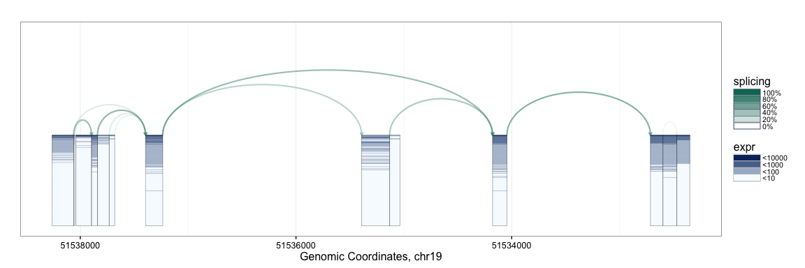
In the plot above, each box arranged horizontally corresponds to a contiguous exonic region along the genome. Each box is colored by 177 horizontal lines, showing the expression level for the 177 samples being analyzed. Note that the exons are plotted along genomic coordinates, and log expression is shown in color.
In addition to the boxes, the plot contains arrows which correspond to a splicing events with sufficient support in the data (e.g. at least 8 samples, each with at least 5 reads spanning the splice junction). The arrows are colored such that darker arrows were present in a higher proportion of the 177 samples (scale shown on right).
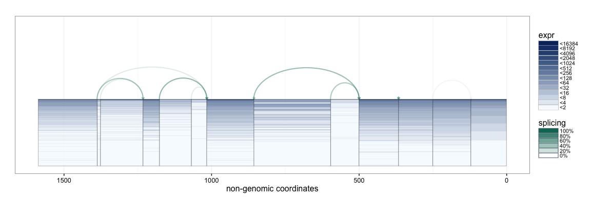
The SpliceGraHM name is in reference to the fact that after removing the spacing between each exon the plot simply reduces to a standard heatmap of expression along a single gene. The corresponding figure after removing the intronic gaps is shown below. The rectangle of color is a heatmap with rows and columns corresponding to samples and exons, respectively.
splicegrahm(klk12_cc, genomic = FALSE, ex_use = 1, log_base = 2)
It is possible to show the coverage of each splice junction using a similar convention with rows corresponding to samples, and with color being used for coverage.
splicegrahm(klk12_cc, genomic = FALSE, j_incl = TRUE)
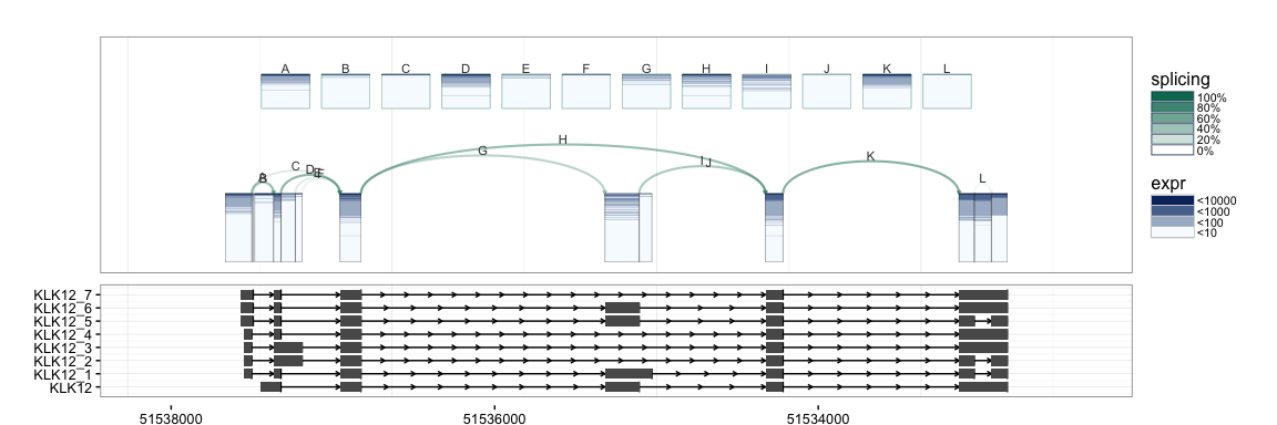
If annotation information is available, e.g. from UCSC KnownGenes, these
can be passed to the function to add an additional track to the plot.
The appropriate GRangesList object to be passed is illustrated in the
following example.
txdb <- TxDb.Hsapiens.UCSC.hg19.knownGene
isActiveSeq(txdb)[seqlevels(txdb)] <- FALSE
isActiveSeq(txdb)[paste0("chr", 1:22)] <- TRUE
exbytx <- exonsBy(txdb, "tx")

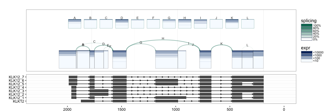
splicegrahm(klk12_cc, genomic = TRUE, j_incl = TRUE, txlist = exbytx)
If gene names are desired, the following can be used to match the
transcript ID in txdb against gene symbols (e.g. in org.Hs.eg.db).
suppressPackageStartupMessages(library("org.Hs.eg.db"))

splicegrahm(klk12_cc, genomic = TRUE, j_incl = TRUE, txlist = exbytx,
            txdb = txdb, orgdb = org.Hs.eg.db)
The splicegrahm function can now also plot gene models in non-genomic
space with an additional parameter eps. The eps parameter determines
how far up/down from the connected component to lookfor overlapping gene
models. If eps = NULL, all overlapping gene models are included. If
eps = 1000, only overlapping gene models which are fully contained
within 1000bp of the connected component are included.
splicegrahm(klk12_cc, genomic = FALSE, j_incl = TRUE, txlist = exbytx,
            txdb = txdb, orgdb = org.Hs.eg.db, eps = NULL)
splicegrahm(klk12_cc, genomic = FALSE, j_incl = TRUE, txlist = exbytx,
            txdb = txdb, orgdb = org.Hs.eg.db, eps = 1)
splicegrahm(klk12_cc, genomic = FALSE, j_incl = TRUE, txlist = exbytx,
            txdb = txdb, orgdb = org.Hs.eg.db, eps = 1000)
Principal Component Analysis (PCA) is a popular exploratory analysis
tool for studying low rank structure in high-dimensional datasets by
projecting the data along the directions of greatest variation. These
directions of greatest variation are often referred to as the PC
"loading" directions. The splicepca function is written to visualize
the loading vectors of splicing data.
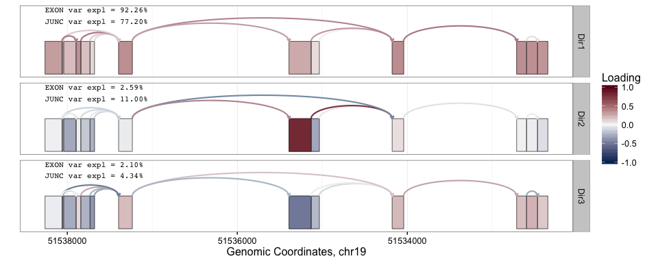
As an example, the following code can be used to visualize the first 3 PC loadings in the KLK12 dataset from above.
splicepca(klk12_cc, npc = 3)
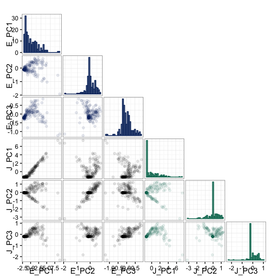
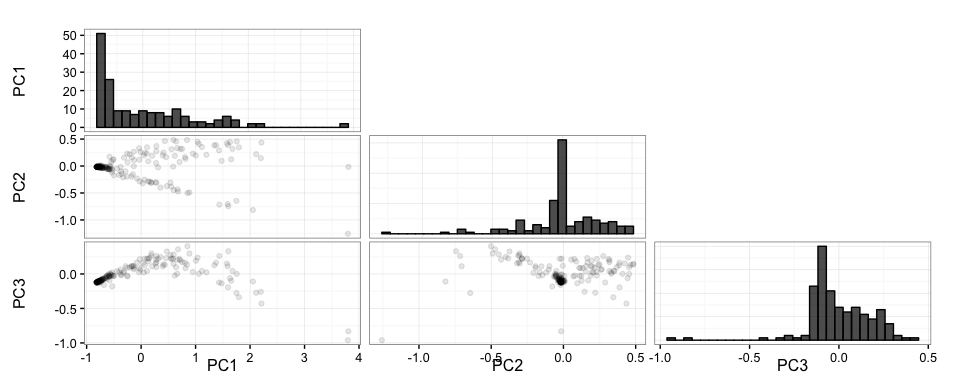
In the above PC loadings plot, red and blue are used to denote the magnitude of the PC loadings for each exon and splice junction. From the plot above, we see that the greatest source of variation in expression at the KLK12 gene locus is the overall expression of the gene. However, the second PC loading shows interesting behavior where the primary source of variation is attributable to the expression of the central exon. Scrolling up a little to the UCSC KnownGenes shown included above, we see that the presence or absence of the central exon actually corresponds to differing isoforms annotated to this gene. Note that above the PCs are computed separately for exons and junctions information. As such, we obtain separate PC "scores" for the exon and junction PC loadings.
splicepca(klk12_cc, npc = 3, scores = TRUE)
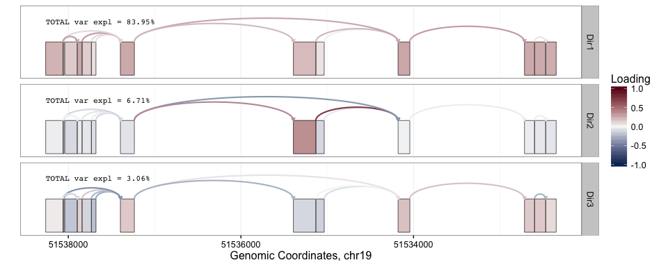
It is also possible to perform the PCA analysis using the concatenated
exon and junction information by setting the pc_sep parameter to
FALSE, and specifying the relative "weight" of each with ej_w. The
exon and junction data are rescaled to each have sum-of-squares equal to
the values specified by ej_w. In the following example, we use equal
weights for the two data sources.
splicepca(klk12_cc, npc = 3, pc_sep = FALSE, ej_w = c(1, 1))
splicepca(klk12_cc, npc = 3, pc_sep = FALSE, ej_w = c(1, 1), scores = TRUE)
All above plots have used color to represent expression. However, low
frequency or outlier events may become lost in this particular view. To
handle this problem, we also provide the option to plot the splicing
objects with vertical height (the y-axis) corresponding to expression.
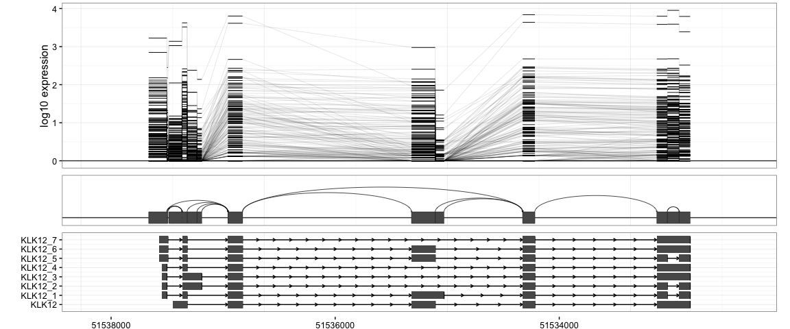
The name of the function is a reference to parallel coordinates
plots. The same KLK12 data is shown below using the splicepcp
function.
splicepcp(klk12_cc, genomic = TRUE, txlist = exbytx, txdb = txdb, orgdb = org.Hs.eg.db)
The plot includes 3 tracks: 1. log-expression values for each exon or region of an exon 2. the complete gene model and splice junctions 3. annotated transcripts from the UCSC KnownGene database.
Currently, the function is being rewritten to also include junction coverage using a parallel coordinates plot in a separate track.
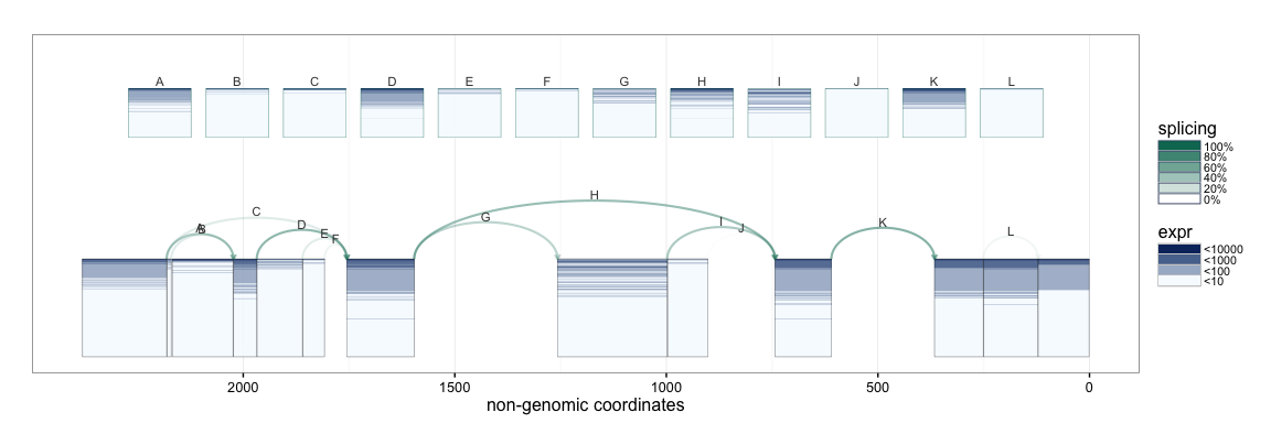
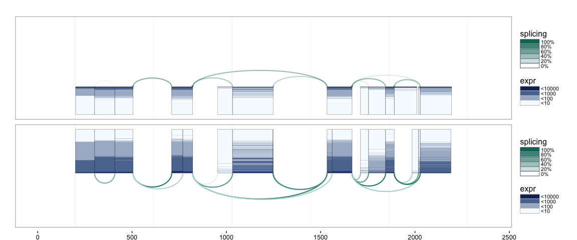
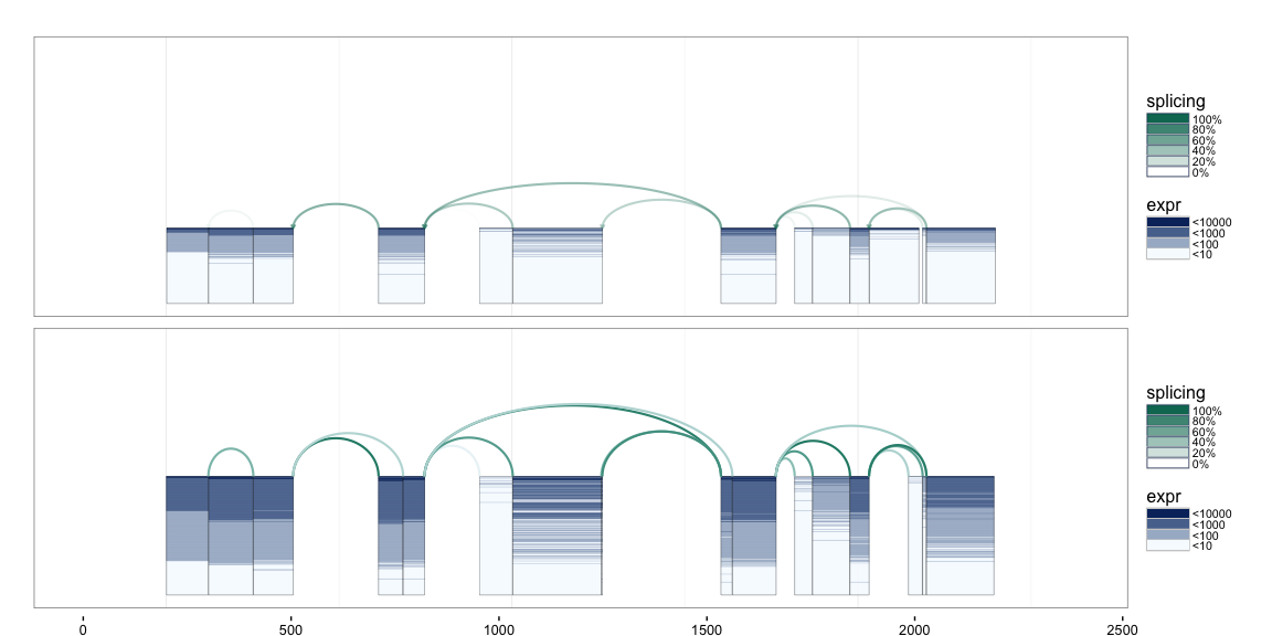
To make direct comparison of two populations possible, we have created
splicegrahm2 which draws two splicegrahm plots in a single figure.
Consider, for example, the task of comparing the behavior of splicing
between the LUSC samples and head and neck squamous cell carcinoma
(HNSC) samples. We have loaded a connected component for 279 HNSC
samples as klk12_hnsc_cc.
data("klk12_hnsc_cc")

splicegrahm2(klk12_cc, klk12_hnsc_cc, genomic=FALSE)
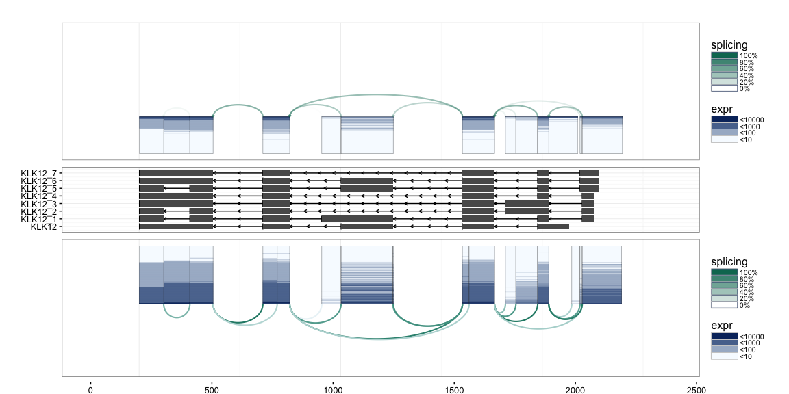
When gene models are also desired, they are placed in a central track
for easy comparison to the two splicegrahms.
splicegrahm2(klk12_cc, klk12_hnsc_cc, genomic=FALSE,
             txlist = exbytx, txdb = txdb, orgdb = org.Hs.eg.db)
Alternatively, the bottom plot can be drawn with the same orientation as
the top plot by setting mirror=FALSE.
splicegrahm2(klk12_cc, klk12_hnsc_cc, genomic=FALSE, mirror=FALSE)
While not modified above, the option same_scale can be used to specify
whether the two plots should be drawn using the same or separate scale
along the y-axis. This can be helpful when the two populations are of
substantially different sizes.
sessionInfo()

## R version 3.3.1 (2016-06-21)
## Platform: x86_64-apple-darwin15.5.0 (64-bit)
## Running under: OS X 10.11.5 (El Capitan)
##
## locale:
## [1] en_US.UTF-8/en_US.UTF-8/en_US.UTF-8/C/en_US.UTF-8/en_US.UTF-8
##
## attached base packages:
## [1] stats4    parallel  stats     graphics  grDevices utils     datasets
## [8] methods   base
##
## other attached packages:
##  [1] spliceclust_1.1.6
##  [2] org.Hs.eg.db_3.3.0
##  [3] BSgenome.Hsapiens.UCSC.hg19_1.4.0
##  [4] BSgenome_1.40.1
##  [5] rtracklayer_1.32.2
##  [6] Biostrings_2.40.2
##  [7] XVector_0.12.1
##  [8] TxDb.Hsapiens.UCSC.hg19.knownGene_3.2.2
##  [9] GenomicFeatures_1.24.5
## [10] AnnotationDbi_1.36.0
## [11] Biobase_2.32.0
## [12] GenomicRanges_1.24.3
## [13] GenomeInfoDb_1.8.7
## [14] IRanges_2.6.1
## [15] S4Vectors_0.10.3
## [16] BiocGenerics_0.18.0
##
## loaded via a namespace (and not attached):
##  [1] httr_1.2.1                    AnnotationHub_2.4.2
##  [3] splines_3.3.1                 Formula_1.2-1
##  [5] shiny_0.14.2                  assertthat_0.1
##  [7] interactiveDisplayBase_1.10.3 latticeExtra_0.6-28
##  [9] RBGL_1.48.1                   Rsamtools_1.24.0
## [11] RSQLite_1.0.0                 lattice_0.20-34
## [13] biovizBase_1.20.0             chron_2.3-47
## [15] digest_0.6.10                 RColorBrewer_1.1-2
## [17] colorspace_1.2-7              ggbio_1.20.2
## [19] htmltools_0.3.5               httpuv_1.3.3
## [21] Matrix_1.2-7.1                plyr_1.8.4
## [23] OrganismDbi_1.14.1            XML_3.98-1.4
## [25] devtools_1.12.0               biomaRt_2.28.0
## [27] zlibbioc_1.18.0               xtable_1.8-2
## [29] scales_0.4.0                  BiocParallel_1.6.6
## [31] htmlTable_1.7                 tibble_1.2
## [33] ggplot2_2.1.0                 withr_1.0.2
## [35] SummarizedExperiment_1.2.3    nnet_7.3-12
## [37] crayon_1.3.2                  mime_0.5
## [39] survival_2.40-1               magrittr_1.5
## [41] memoise_1.0.0                 evaluate_0.10
## [43] GGally_1.2.0                  foreign_0.8-67
## [45] graph_1.50.0                  BiocInstaller_1.24.0
## [47] tools_3.3.1                   data.table_1.9.6
## [49] formatR_1.4                   stringr_1.1.0
## [51] munsell_0.4.3                 cluster_2.0.5
## [53] ensembldb_1.4.7               compiler_3.3.1
## [55] grid_3.3.1                    RCurl_1.95-4.8
## [57] dichromat_2.0-0               VariantAnnotation_1.18.7
## [59] labeling_0.3                  bitops_1.0-6
## [61] rmarkdown_1.1                 testthat_1.0.2
## [63] gtable_0.2.0                  DBI_0.5-1
## [65] reshape_0.8.6                 roxygen2_5.0.1
## [67] reshape2_1.4.2                R6_2.2.0
## [69] GenomicAlignments_1.8.4       gridExtra_2.2.1
## [71] knitr_1.14                    Hmisc_4.0-0
## [73] stringi_1.1.2                 Rcpp_0.12.7
## [75] rpart_4.1-10                  acepack_1.4.1
