The pretrends package provides tools for power calculations for
pre-trends tests, and visualization of possible violations of parallel
trends. Calculations are based on Roth (2022).
This is the Stata version of the R package of the same name.
(Please cite the paper if you enjoy the package!)
If you’re not an R or Stata user, you may also be interested in the associated Shiny app.
version 0.4.3 09Oct2023 | Installation | Application
The package may be installed by using net install:
local github https://raw.githubusercontent.com
net install pretrends, from(`github'/mcaceresb/stata-pretrends/main) replace
You can also clone or download the code manually, e.g. to
stata-pretrends-main, and install from a local folder:
cap noi net uninstall pretrends
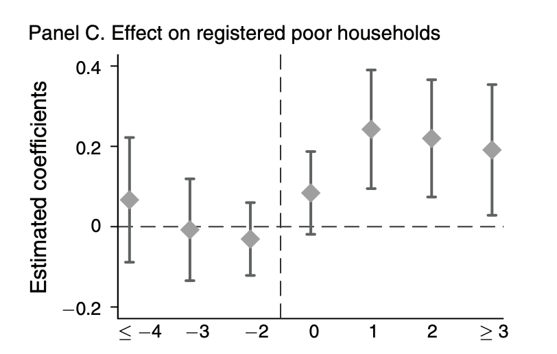
net install pretrends, from(`c(pwd)'/stata-pretrends-main)We illustrate how to use the package with an application to He and Wang (2017). The analysis will be based on the event-study in Figure 2C, which looks like this:
We first load the dataset used by He and Wang.
use "https://media.githubusercontent.com/media/mcaceresb/stata-pretrends/main/data/workfile_AEJ.dta", clearWe then run their regression specification.
reghdfe l_poor_reg_rate Lead_D4_plus Lead_D3 Lead_D2 D0 Lag_D1 Lag_D2 Lag_D3_plus, absorb(v_id year) cluster(v_id)which yields the following results
             |               Robust
l_poor_reg~e | Coefficient  std. err.      t    P>|t|     [95% conf. interval]
-------------+----------------------------------------------------------------
Lead_D4_plus |   .0667032   .0897108     0.74   0.458    -.1099686    .2433749
     Lead_D3 |  -.0077018   .0732436    -0.11   0.916     -.151944    .1365404
     Lead_D2 |  -.0307691   .0523996    -0.59   0.558    -.1339621     .072424
          D0 |   .0840307   .0595518     1.41   0.159    -.0332475    .2013088
      Lag_D1 |   .2424418   .0853721     2.84   0.005     .0743146    .4105691
      Lag_D2 |    .219879    .084391     2.61   0.010     .0536838    .3860741
 Lag_D3_plus |   .1910925   .0940472     2.03   0.043     .0058809    .3763042
       _cons |   1.478639   .0771617    19.16   0.000      1.32668    1.630597
In this case, these coefficients come from a two-way fixed effects regression using reghdfe. However, the pretrends package will work with any package that produces an event-study from any
asymptotically normal estimator, including
Callaway and Sant’Anna (2020)
and Sun and Abraham (2020), so long as the resulting estimates and coefficients are saved in e(b) and e(V). If one is using a command that does not export an e(b) and e(V), one can instead provide the coefficients and covariance matrix directly via the beta() and vcov() options.
The package has two subcommands:
-
The
powersub-command calculates the slope of a linear violation of parallel trends that a pre-trends test would detect a specified fraction of the time. (By detect, we mean that there is any significant pre-treatment coefficient.) -
Alternatively, the user can specify a hypothesized violations of parallel trends—the package then creates a plot to visualize the results, and reports various statistics related to the hypothesized difference in trend. The user can specify a hypothesized linear pre-trend via the
slope()option, or provide an arbitrary violation of parallel trends via thedelta()option.
Let's illustrate the first use case:
pretrends power 0.5, pre(1/3) post(4/7)

* Slope for 50% power =  .0494932

return list
* scalars:
*               r(slope) =  .0494932155202119
*               r(Power) =  .5
In the command above, the option pre(1/3) tells the package that the pre-treatment event-study coefficients are in positions 1 through 3 in our regression results. (The package assumes that the period before the event-study is normalized to zero and omitted from the regression.) Likewise, the option post(4/7) tells the package that the post-treatment coefficients are in positions 4 through 7. The results of the command tells us that if there was a linear violation of parallel trends with slope 0.049, then we would have 50% power to detect it (where we say it's "detected" if there is a significant pre-trend coefficient). If we want wanted a different power threshold, say 80%, we would change power 0.5 to power 0.8 in the command above.
Next, we illustrate how to visualize violations of parallel trends using the package's second subcommand. For simplicitly, lets visualize the linear trend against which pre-tests have 50 percent power that we just calculated. This is just for illustration—you can visualize any violation that you want, and should choose an economically relevant one. To do this, we run the command:
matrix sigma = e(V)
matrix beta  = e(b)
matrix beta  = beta[., 1..7]
matrix sigma = sigma[1..7, 1..7]
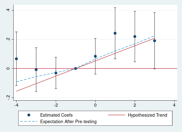
pretrends, numpre(3) b(beta) v(sigma) slope(`r(slope)')
This tells Stata to visualize a linear violation of parallel trends with slope r(slope), i.e. the value calculated by the previous command (0.049). If you wanted to visualize a linear violation with slope 5, you'd just specify slope(5). (Note when specifying numpre() the vector b() and the matrix v() must only contain the relevant coefficients.) The resulting plot super-imposes the conjectured linear violation of parallel trends on the event-plot in red. It also shows in dashed blue what we'd expect the coefficients to look like on average conditional on not finding a significant pre-trend if in fact that truth was the hypothesized red line. In the plot above, both the red line and blue line are contained within all of the confidence intervals (with the exception of one pre-period for the red line), so the hypothesized trend seems somewhat plausible.
Note that to create the plot above, the coefplot package is required; if the coefplot package is not
installed or not available, the user can add option nocoefplot to
skip the visualization. In either case the event study data is saved in
r(), along several useful statistics about the power of the pre-test
against the hypothesized trend.
* data for visualization
matlist r(results)
*          r1 |        -4   .0667032  -.1091268   .2425331  -.1484796   -.087755
*          r2 |        -3  -.0077018  -.1512567   .1358531  -.0989864   -.052812
*          r3 |        -2  -.0307691  -.1334704   .0719323  -.0494932  -.0265324
*          r4 |        -1          0          0          0          0          0
*          r5 |         0   .0840307  -.0326887     .20075   .0494932   .0617067
*          r6 |         1   .2424418   .0751157    .409768   .0989864   .1148959
*          r7 |         2    .219879   .0544757   .3852823   .1484796   .1611171
*          r8 |         3   .1910925   .0067634   .3754217   .1979729   .2134771


return list
* scalars:
*               r(LR) =  .1016996725963556
*               r(Bayes) =  .5690176868657252
*               r(Power) =  .5000000000010103
*               r(slope) =  .0494932155202119
*
* macros:
*    r(PreTrendsResults) : "PreTrendsResults"
*
* matrices:
*             r(results) :  8 x 6
*               r(delta) :  1 x 8
An explanation of the returned results is as follows:
-
r(results) The data used to make the event plot. Note the column
meanAfterPretesting, which is also plotted, shows the expected value of the coefficients conditional on passing the pre-test under the hypothesized trend (i.e. what's shown in the blue dashed line). -
r(Power) The probability that we would find a significant pre-trend under the hypothesized pre-trend. (This is 0.50, up to numerical precision error, by construction in our example). If you hypothesize a different trend, it may be something different.
-
r(BF) (Bayes Factor) The ratio of the probability of "passing" the pre-test under the hypothesized trend relative to under parallel trends. Here, the probability of passing the pre-test under the hypothesized trend is about half as likely (56%) as it is under parallel trends.
-
r(LR) (Likelihood Ratio) The ratio of the likelihood of the observed pre-treatment coefficients under the hypothesized trend relative to under parallel trends. Here, the realization of the pre-trends is about 1/10th as likely under the hypothesized trend as under parallel trends.
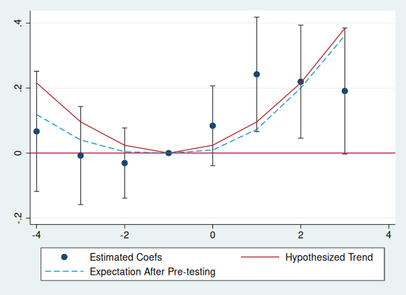
Last, although our example has focused on a linear violation of parallel trends, the package allows the user to input an arbitrary non-linear hypothesized trend. For instance, here is the event-plot and power analysis from a quadratic trend.
mata st_matrix("deltaquad", 0.024 * ((-4::3) :- (-1)):^2)
pretrends, time(-4(1)3) ref(-1) deltatrue(deltaquad) coefplot
matlist r(results)
* | t betahat lb ub deltatrue meanAft~g
* -------------+------------------------------------------------------------------
* r1 | -4 .0667032 -.1091268 .2425331 .216 .1157555
* r2 | -3 -.0077018 -.1512567 .1358531 .096 .0391983
* r3 | -2 -.0307691 -.1334704 .0719323 .024 .003749
* r4 | -1 0 0 0 0 0
* r5 | 0 .0840307 -.0326887 .20075 .024 .0089854
* r6 | 1 .2424418 .0751157 .409768 .096 .0723966
* r7 | 2 .219879 .0544757 .3852823 .216 .2000759
* r8 | 3 .1910925 .0067634 .3754217 .384 .3612036
return list
* scalars:
* r(LR) = .3962795305253372
* r(Bayes) = .3384376031301103
* r(Power) = .7026124047271576
*
* macros:
* r(PreTrendsResults) : "PreTrendsResults"
*
* matrices:
* r(results) : 8 x 6
* r(delta) : 1 x 8(Note when specifying time() and ref()' by default the vector b() and the matrix v() must start with the relevant coefficients. The number of pre-period is taken to be the number of entries in the time vector strictly smaller than ref(), and the number of post-periods the number of entries strictly larger. time() and ref() may be combined with pre() and post(); numpre() may not be combined with either.)


