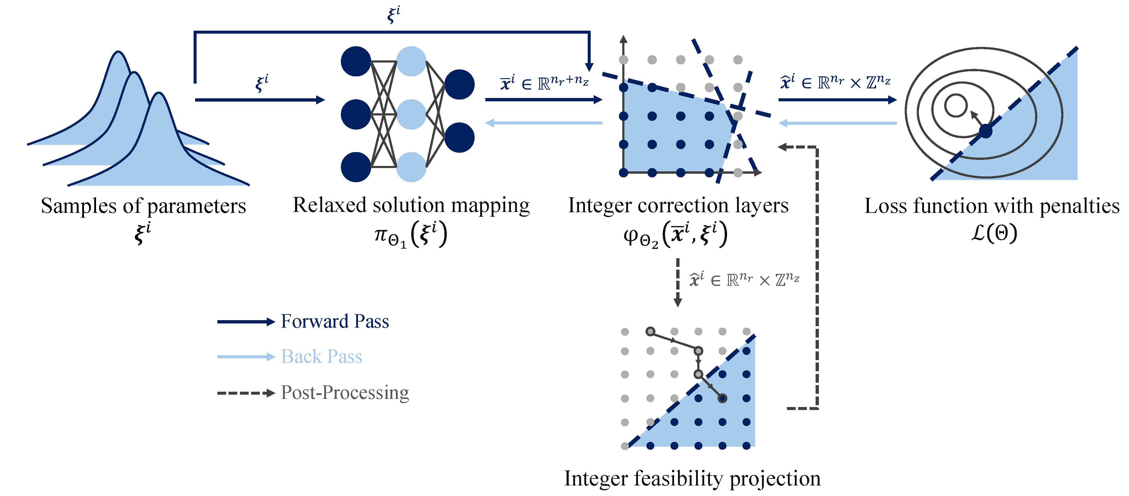
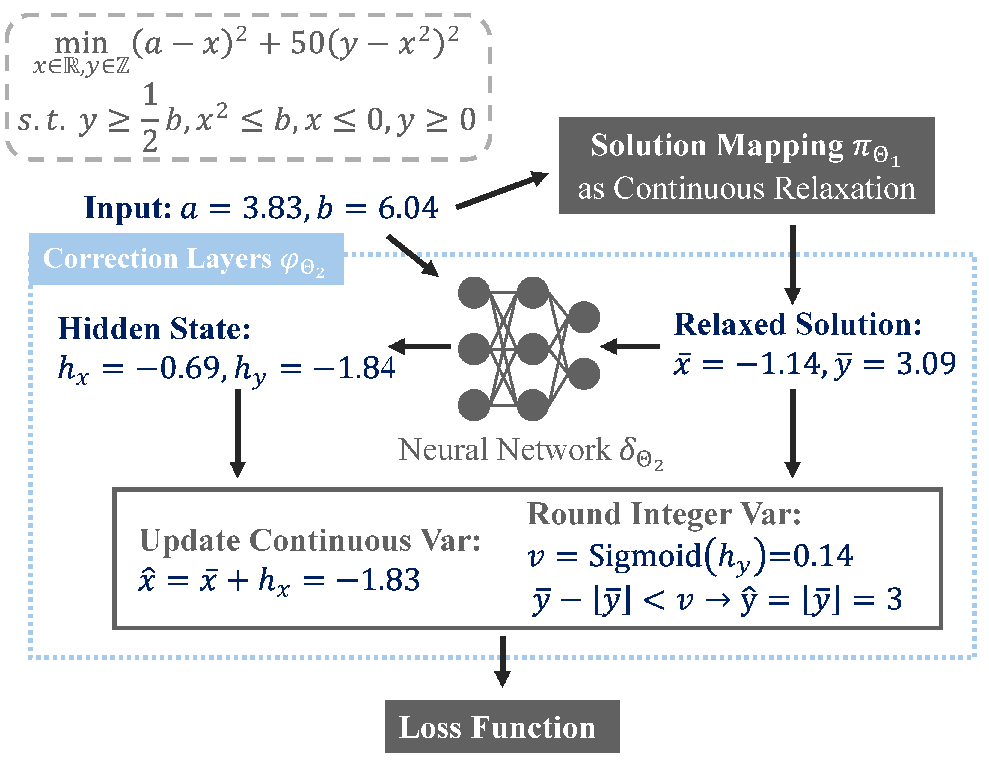
This project is an implementation of Differentiable Mixed-Integer Programming Layers based on the NeuroMANCER library. It introduces learnable differentiable correction layers for rounding and projection, enabling efficient integer solution acquisition for parametric nonlinear mixed-integer problems through neural networks, thus eliminating the need for traditional mathematical programming solvers.
While inherently heuristic and not guaranteed to find the optimal or even a feasible solution, the framework often provides high-quality feasible solutions that are extremely useful either as alternatives to optimal solutions or as initial solutions for traditional solvers. This capability makes them invaluable tools in complex optimization scenarios where exact methods might struggle or be too slow.
-
Efficient Solution Acquisition: The entire solution process relies entirely on neural networks without the need for mathematical programming solvers.
-
Integer Solution Guarantee: Integrates learnable rounding directly into the network architecture, ensuring that solutions adhere strictly to integer constraints.
A generic formulation of a multiparametric mix-integer nonlinear program (pMINLP) is given in the form:
where
To run this project, you will need the following libraries and software installed:
- Python: The project is developed using Python. Ensure you have Python 3.9 or later installed.
- Scikit-Learn: Useful for performing various machine learning tasks.
- PyTorch: Used for building and training neural network models.
- NumPy: Essential for numerical operations.
- Pandas: Useful for data manipulation and analysis.
- Pyomo: A Python library for optimization modeling.
- SCIP: A powerful solver for mathematical programming, which might need a separate installation process.
- Neuromancer: This project uses the Neuromancer library for differentiable programming.
├── archive                        # Archive for older files and documents
├── img                            # Image resources for the project
├── src                            # Main source code directory
│   ├── __init__.py                # Initializes the src package
│   ├── func                       # Directory for function modules
│       ├── __init__.py            # Initializes the function submodule
│       ├── layer.py               # Pre-defined neural network layers
│       ├── ste.py                 # Straight-through estimators for non-differentiable operations
│       ├── rnd.py                 # Modules for differentiable and learnable rounding
│       └── proj.py                # Modules for differentiable and learnable projection
│   ├── problem                    # Modules for the benchmark of constrained optimization
│       ├── __init__.py            # Initializes the problem submodule
│       ├── math_solver            # Collection of Predefined SCIP solvers
│           ├── __init__.py        # Initializes the mathematical solver submodule
│           ├── abc_solver.py      # Abstract base class for solver implementations
│           ├── quadratic.py       # SCIP model for MIQP
│           └── rosenbrock.py      # SCIP model for MIRosenbrock
│       └── neuromancer            # Collection of Predefined NeuroMANCER maps
│           ├── __init__.py        # Initializes the NeuroMANCER map submodule
│           ├── quadratic.py       # NeuroMANCER map for MIQP
│           └── rosenbrock.py      # NeuroMANCER map for MIRosenbrock
│   └── utlis                      # Utility tools such as data processing and result test
│       ├── __init__.py            # Initializes the utility submodule
│       └── data.py                # Data processing file
│       └── solve_test.py          # Testing functions to evaluate optimization solution
├── sweep_QP-Round.py              # Script for hyperparameter tuning for MIQP
├── sweep_Rosenbrock-Round.py      # Script for hyperparameter tuning for MIRosenbrock
└── README.md                      # README file for the project
These algorithms provide mechanisms for rounding within a differentiable programming framework, addressing the challenge of non-differentiable operations inherent in discrete optimization. They are crucial in scenarios where solutions must adhere to integer output with constraints.
The algorithm starts with a relaxed solution
During the training of neural networks, non-differentiable operations such as binarization, flooring, and indicator functions pose significant challenges for gradient-based optimization methods because these functions lost gradients. To avoid these issues, the straight-through estimator (STE) is employed. This approach allows the gradient of a rounded result to pass through unaltered from its input, effectively enabling optimization of functions that involve non-differentiable transformations.
This algorithm is specifically designed to adaptively decide the rounding direction—whether to round up (ceiling) or down (floor)—for each variable based on the contextual data it processes.
The diffGumbelBinarize, as implemented, utilizes the Gumbel-Softmax distribution to introduce two Gumbel noises into the logits of 0 and 1 during the training. This approach simulates the randomness associated with rounding decisions, and by adjusting the temperature parameter, it controls the sharpness of the binarization, effectively balancing exploration and exploitation in the rounding process.
This algorithm introduces a dynamic, learnable threshold that determines the specific rounding behavior for each integer variable.
These algorithms aim to reduce constraint violation. The projection is applied iteratively for a predefined number of steps
This algorithm is designed to refine solutions to ensure they adhere to the defined constraints by repeatedly projecting onto a feasible region.
Extending the concept of projected gradients, this algorithm incorporates a solution mapping phase that predicts residuals used to adjust the solution before projection.
A parametric MIQP model with both continuous variables
In this formulation, the objective function is a quadratic function of
The fixed parameters of an example from A multiparametric programming approach for mixed-integer quadratic engineering problems, are defined as follows:
The variable parameter
The parametric, high-dimension, Integer, and constrained Rosenbrock problem implemented in this project serves as a rigorous testbed for evaluating the efficacy of our differentiable programming framework, in which
The scalar parameter
Here is a simple example demonstrating learnable rounding within a neural network framework:
# get objective function & constraints
from src.problem import nmQuadratic
obj, constrs = nmQuadratic(["x_rnd"], ["p"], penalty_weight=10)

# define neural architecture for the solution map
import neuromancer as nm
func = nm.modules.blocks.MLP(insize=2, outsize=4, bias=True,
                             linear_map=nm.slim.maps["linear"],
                             nonlin=nn.ReLU, hsizes=[10]*4)
smap = nm.system.Node(func, ["p"], ["x"], name="smap")

# define rounding model using Gumbel binarization
from src.func.layer import netFC
layers_rnd = netFC(input_dim=6, hidden_dims=[20]*3, output_dim=4)
from src.func.rnd import roundGumbelModel
round_func = roundGumbelModel(layers=layers_rnd, param_keys=["p"], var_keys=["x"], output_keys=["x_rnd"],
                              bin_ind={"x":[2,3]}, continuous_update=False, name="round")


# construct the complete neuromancer problem with all components
components = [smap, round_func]
loss = nm.loss.PenaltyLoss(obj, constrs)
problem = nm.problem.Problem(components, loss)Here is a simple example demonstrating learnable projection within a neural network framework:
# get objective function & constraints
from src.problem import nmQuadratic
obj_bar, constrs_bar = nmQuadratic(["x_bar"], ["p"], penalty_weight=10)
obj_rnd, constrs_rnd = nmQuadratic(["x_rnd"], ["p"], penalty_weight=10)

# define neural architecture for the solution map
import neuromancer as nm
func = nm.modules.blocks.MLP(insize=2, outsize=4, bias=True,
                             linear_map=nm.slim.maps["linear"],
                             nonlin=nn.ReLU, hsizes=[10]*4)
smap = nm.system.Node(func, ["p"], ["x"], name="smap")

# define rounding layer using Gumbel binarization
from src.func.layer import netFC
layers_rnd = netFC(input_dim=6, hidden_dims=[20]*3, output_dim=4)
from src.func.rnd import roundGumbelModel
round_func = roundGumbelModel(layers=layers_rnd, param_keys=["p"], var_keys=["x"], output_keys=["x_rnd"],
                              bin_ind={"x":[2,3]}, continuous_update=False, name="round")


# define projection layer with specified parameters
num_steps = 10
step_size = 0.1
decay = 0.1
layers_proj = netFC(input_dim=10, hidden_dims=[20]*3, output_dim=4)
from src.func.proj import solPredGradProj
proj = solPredGradProj(layers=layers_proj, constraints=constrs_bar, param_keys=["p"],
                       var_keys=["x_rnd"], output_keys=["x_bar"], num_steps=num_steps,
                       step_size=step_size, decay=decay)

# construct the complete neuromancer problem with all components
components = [smap, round_func, proj]
loss = nm.loss.PenaltyLoss(obj_bar, constrs_bar)
problem = nm.problem.Problem(components, loss, grad_inference=True)


