- cmd/anomaly_bench - Anomaly detection for JSON documents prototype code
- cmd/anomaly_image - Anomaly detection for images
- cmd/lstm - LSTM test code
- cmd/search_lfsr - Code for finding maximal length lfsr
- images - Test images for anomaly_image
- lstm - LSTM implementation
- gru - GRU implementation
Standard statistical methods can be used for anomaly detection of one dimensional real valued data. The multidimensional nature of JSON documents makes anomaly detection more difficult. Firstly, this README proposes a two stage algorithm for the anomaly detection of JSON documents. The first stage of the algorithm uses random matrix dimensionality reduction to vectorize a JSON document into a fixed length vector (JSON document vector). The second stage of the algorithm uses one of three methods: average cosine similarity, a single neuron, or an autoencoder to determine how surprising the JSON document vector is. Secondly, this README proposes using a LSTM or a GRU recurrent neural network for anomaly detection. Thirdly, a probabilistic model based on models for adaptive arithmetic coding and Kolmogorov complexity is proposed. Fourthly, a probabilistic model with resampling is proposed. Simple statistical analysis can then be used for determining which JSON documents the user should be alerted to.
The typical approach for converting a document into a vector is to count words. Each entry in the vector corresponds to the count for a particular word. In order to capture more document struct word pairs could be counted instead. JSON documents have explicit struct that should be captured in the computed vector. For example the below JSON:
{
 "a": [
  {"a": "aa"},
  {"b": "bb"}
 ],
 "b": [
  {"a": "aa"},
  {"b": "bb"}
 ]
}
would be converted into the below 12 "words" using a recursive algorithm:
- a a aa
- a aa
- aa
- a b bb
- b bb
- bb
- b a aa
- a aa
- aa
- b b bb
- b bb
- bb
The 8 unique words are ["a a aa", "a aa", "aa", "a b bb", "b bb", "bb", "b a aa", "b b bb"], and their vector is [1, 2, 2, 1, 2, 2, 1, 1]. For all possible JSON documents the vector would be very large, so an algorithm is needed for compressing this vector.
Dimensionality reduction compresses a large vector into a smaller vector. This is done by multiplying a vector by a matrix. Principal component analysis (PCA) is the algorithm typically used, but it doesn't scale well for larger vectors. For very large vectors a random matrix can be used instead of a matrix generated by PCA. The random matrix is filled with (-1, 1, 0) with respective odds (1/6, 1/6, 4/6). For the vector from the previous section the matrix would look like: [0 1 0 0 -1 0 0 1; 1 0 0 -1 0 1 0 0]. This matrix would compress the 8 entry vector down to a 2 entry vector. As an optimization the matrix columns can be generated on the fly using a random number generator seeded with the hash of a particular word. Addition can then be used to replace multiplication.
The code for the vectorizer can be found here.
Three anomaly detection methods are described below. Each method computes a surprise metric from a JSON document vector.
The average cosine similarity method works by computing the cosine similarity between a given JSON document vector and each member of a JSON document vector database. The average is then computed. This metric represents how close the given JSON document vector is to the database of document vectors on average. After computing the average cosine similarity the JSON document vector is added to the database. The algorithm gets slower with time.
The code for the average cosine similarity algorithm can be found here.
A single neuron implemented with the cosine similarity formula can be used for anomaly detection. The single valued output of the neuron represents how surprising the inputed JSON document vector is. The single neuron is trained with a JSON document vector as input and 1 as the output.
The code for the single neuron algorithm can be found here.
An autoencoding neural network isn't trained with labeled data, instead it is trained to output the input vector. The standard autoencoder has three layers. The top and bottom layers are the same size, and the middle layer is typically more narrow than the top and bottom layers. The narrow middle layer creates an information bottleneck. It is possible to compute an autoencoder error metric for a particular JSON document vector. This "surprise" metric is computed by inputing the JSON document vector into the neural network and then computing the mean squared error at the output. The neural network can then be trained on the JSON document vector, so the neural network isn't surprised by similar JSON document vectors in the future.
The code for the autoencoder algorithm can be found here.
The LSTM takes a series of bytes as input and outputs a predicted next byte. The LSTM algorithm works by training a LSTM on JSON data. The cost of training is then used as a surprise metric of the JSON data. Unlike the above algorithms, the LSTM based solution is capable of anomaly detection for non-JSON binary protocols. The LSTM has a state which could be used as a JSON document vector as in the above algorithm.
The code for the LSTM algorithm can be found here.
A GRU is similar to a LSTM, but it requires fewer tensor operations. The cost of training is still used as a surprise metric.
The code for the GRU algorithm can be found here.
The complexity algorithm works by computing the compressed bits per symbol of a JSON document given the previous JSON documents. The JSON document isn't compressed, instead the compressed bits per symbol is computed with log2 of the symbol probabilities generated by the model for adaptive arithmetic coding.
The code for the complexity algorithm can be found here.
The complexity with resampling algorithm is implemented with multiple copies of the above complexity model. Each copy sees a subset of the training data set. This allows the uncertainty in surprise to be computed.
The code for the complexity with resampling algorithm can be found here.
The benchmarks are executed with:
go test -bench=.
BenchmarkLFSR-4                    	2000000000	         2.02 ns/op
BenchmarkSource-4                  	500000000	         3.47 ns/op
BenchmarkVectorizer-4              	    2000	    526639 ns/op
BenchmarkVectorizerLFSR-4          	   10000	    103305 ns/op
BenchmarkVectorizerNoCache-4       	    2000	   1069329 ns/op
BenchmarkVectorizerLFSRNoCache-4   	    5000	    200034 ns/op
BenchmarkAverageSimilarity-4       	   10000	   1268110 ns/op
BenchmarkNeuron-4                  	    5000	    231500 ns/op
BenchmarkAutoencoder-4             	     200	   7310656 ns/op
BenchmarkLSTM-4                    	      10	 117217241 ns/op
BenchmarkGRU-4                     	      20	  80982837 ns/op
BenchmarkComplexity-4              	   20000	     96472 ns/op
As can been seen the LSTM based algorithm is much slower than the two stage algorithm. The complexity based approach is the fastest solution.
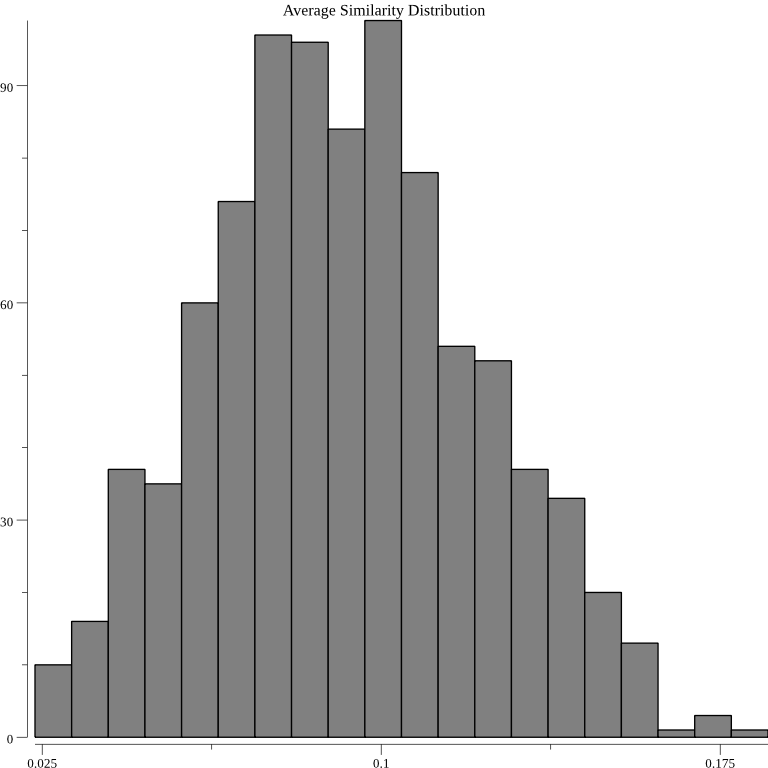
Verification is accomplished by generating random JSON documents from a gaussian random variable and feeding them into the anomaly detection algorithm. The below graph shows the distribution resulting from average cosine similarity method being fed random JSON documents:
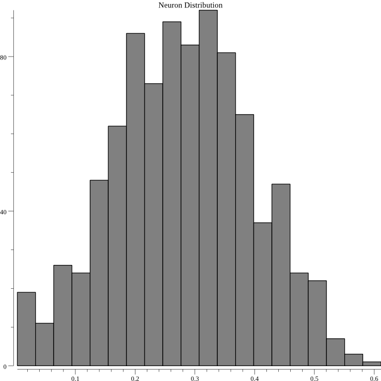
For single neuron:
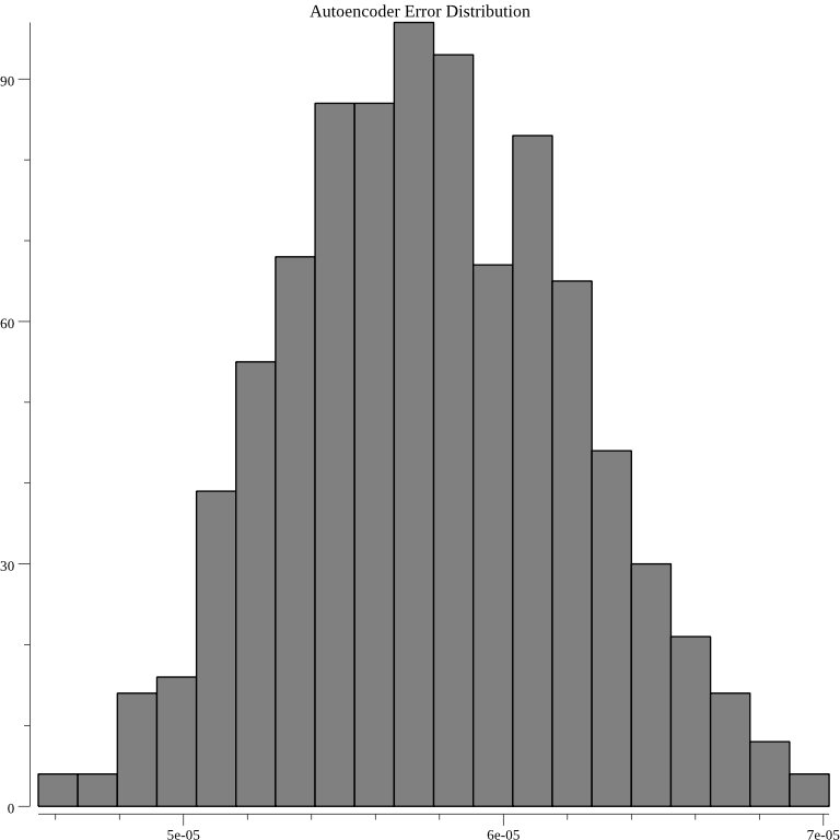
For autoencoder:
As should be expected the graphs appears to be gaussian. Another test implemented feeds the below two JSON documents into each of the above three anomaly detection algorithms after they have been trained on 1000 random JSON documents:
First test JSON document:
{
 "alfa": [
  {"alfa": "1"},
  {"bravo": "2"}
 ],
 "bravo": [
  {"alfa": "3"},
  {"bravo": "4"}
 ]
}
Second test JSON document:
{
 "a": [
  {"a": "aa"},
  {"b": "bb"}
 ],
 "b": [
  {"a": "aa"},
  {"b": "bb"}
 ]
}
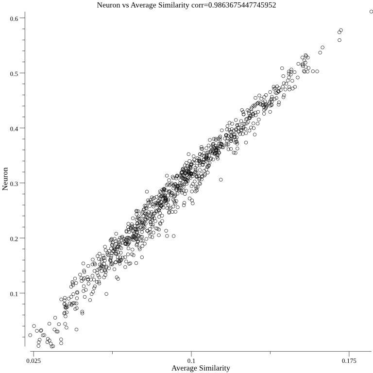
The second JSON document is more similar to the randomly generated JSON documents than the first JSON document. This idea is tested 100 times by changing the random seed used to generate the 1000 random JSON documents. All of the methods pass the test with a score near 100. This shows that the anomaly detection algorithm isn't a random number generator. One final test is performed by graphing the output of the single neuron method and the autoencoder method against the average cosine similarity method. The below graph 5 shows that the output of the single neuron correlates with average cosine similarity:
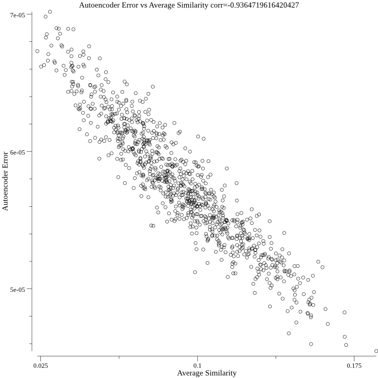
The below graph 8 shows that the autoencoder method correlates with average cosine similarity:
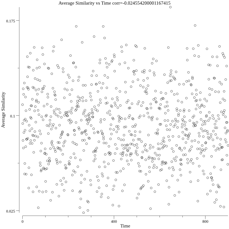
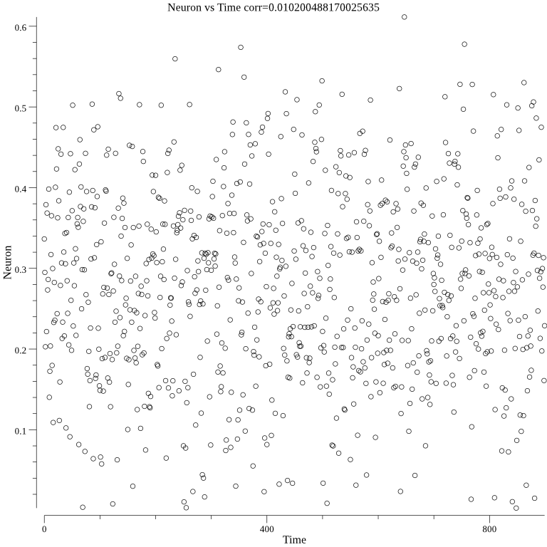
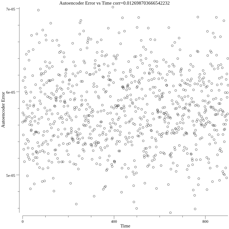
The below three graphs show average cosine similarity, single neuron, and autoencoder are not correlated through time:
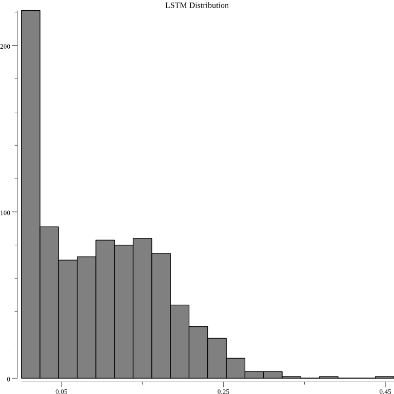
The distribution of the LSTM surprise metrics for random JSON documents is wide:
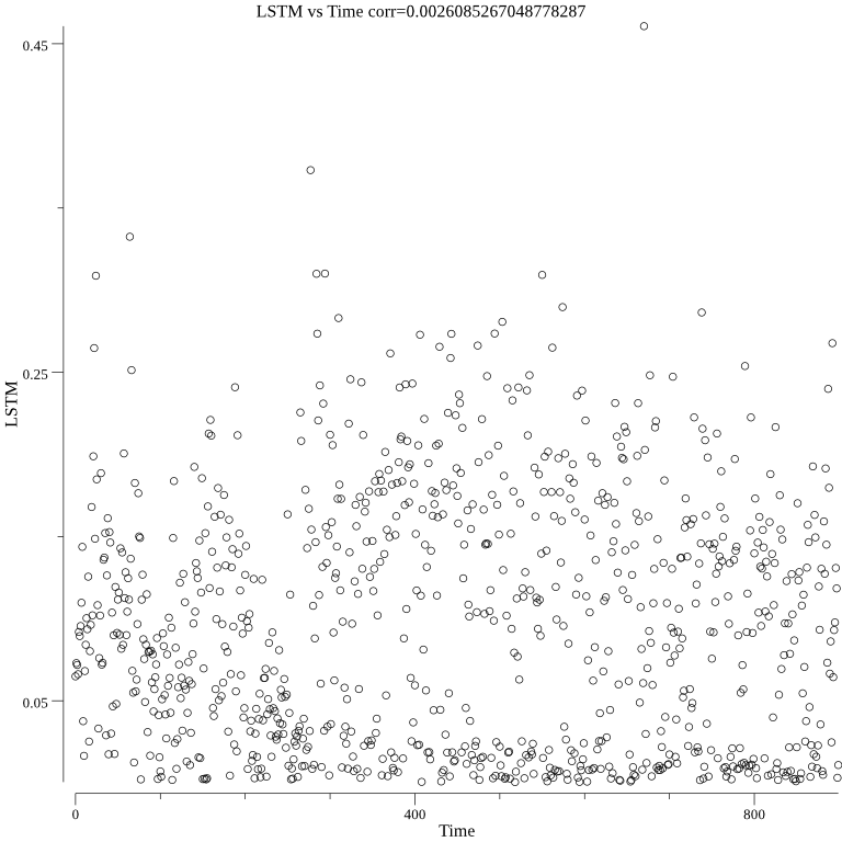
The LSTM over time can be seen in the below graph:
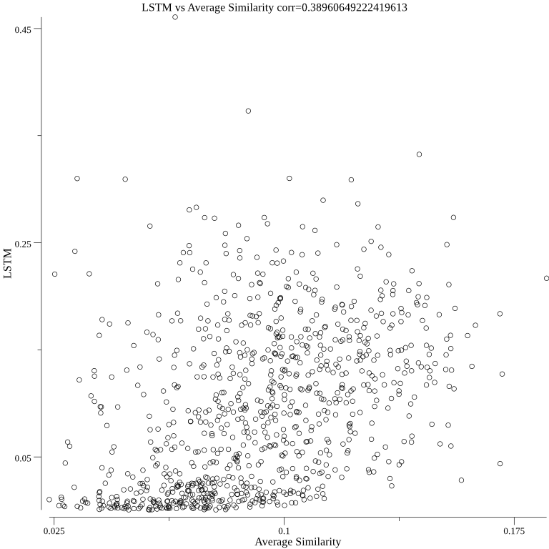
The LSTM algorithm correlates with the average similarity approach:
The LSTM correctly determines the surprise metrics of the above two test JSON documents. The surprise metric of the first test JSON document is greater than the surprise metric of the second test JSON document.
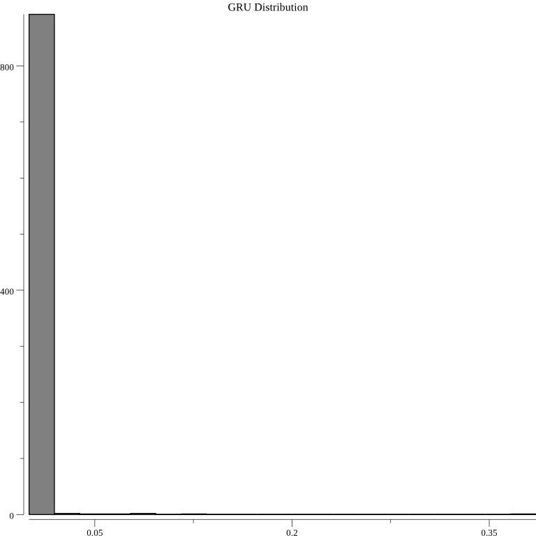
The distribution of the GRU surprise metrics is different from the LSTM distribution:
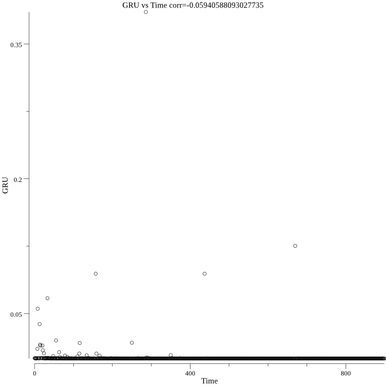
The GRU over time can be seen in the below graph:
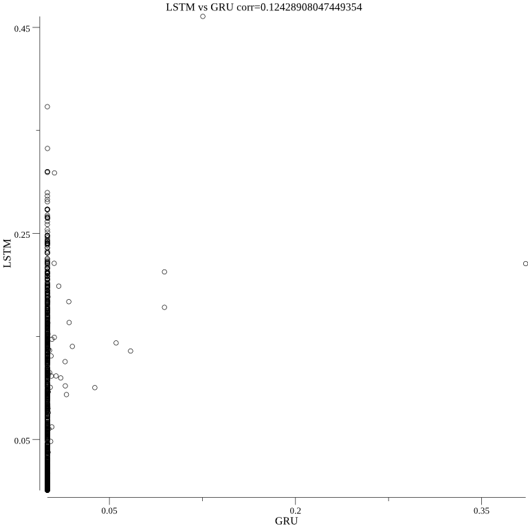
The LSTM and GRU algorithms are correlated. This means that they are probably not computing a random process:
The GRU correctly determines the surprise metrics of the above two test JSON documents. The surprise metric of the first test JSON document is greater than the surprise metric of the second test JSON document.
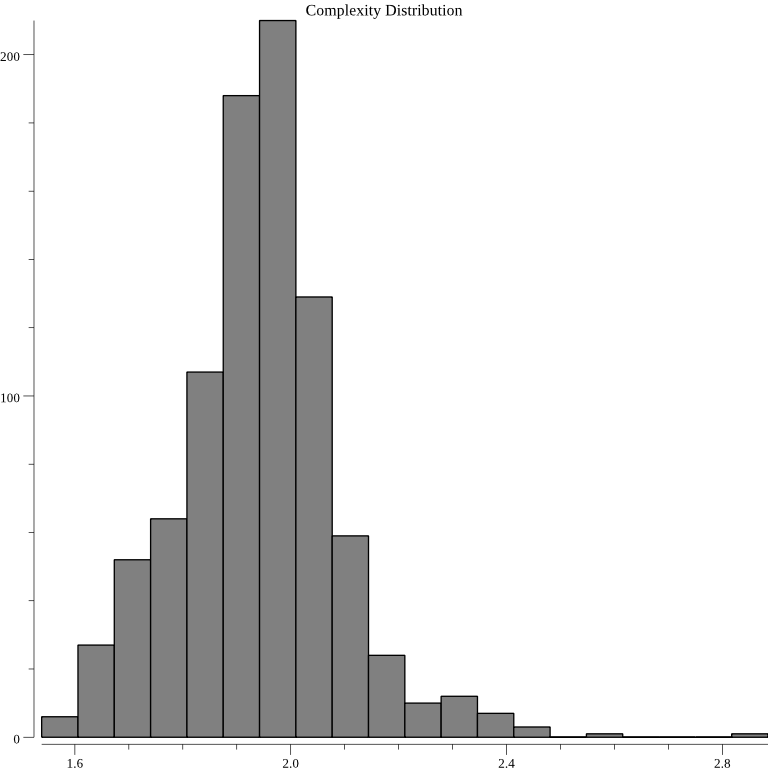
The distribution for the complexity surprise metrics is normal:
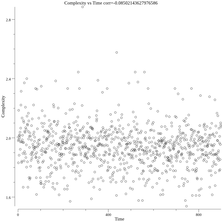
It can be seen that the complexity model learns over time:
The complexity algorithm correctly determines the surprise metrics of the above two test JSON documents. The surprise metric of the first test JSON document is greater than the surprise metric of the second test JSON document.
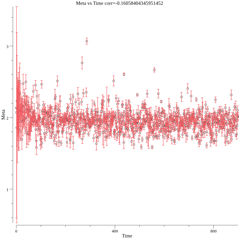
The below graph shows the complexity over time with error bars representing uncertainty:
An anomaly detection engine has been demonstrated. The first two stage algorithm is made up of two components: a vectorizer and an algorithm for computing surprise. After vectorization the single neuron and autoencoder algorithms have a fixed cost for determining if a JSON document is an anomaly. The single neuron and autoencoder methods are suitable for taking a real time learning approach. The single neuron method is faster than the other two methods. The LSTM based algorithm works, but it is slower than the other approaches. A GRU based algorithm can be used instead of a LSTM based algorithm for faster performance. The complexity algorithm is the fastest solution and supports any type of data.
- The LSTM algorithm could be used to replace the vectorizer of the two stage algorithm. In theory this should result in more optimal vectorization.
- Instead of a LSTM based recurrent neural network, a GRU based recurrent neural network could be used. The GRU would be faster than the LSTM.
- Use a recurrent neural network to create a heat map of the JSON document. This would show the parts that are anomalies.
- Ensemble learning could be used to combine multiple algorithms.
- Use models for adaptive arithmetic coding for anomaly detection.
