This repository contains the data and code required to reproduce the results and visualizations from the forthcoming paper "One week ahead prediction of harmful algal blooms in Iowa lakes." Harmful algal blooms occur in freshwater lakes during warmer seasons of the year and cause harm to humans, wildlife, and the surrounding environment. Based on weekly samples collected by the Iowa DNR, we trained several models in order to see how well we could predict harmful algal blooms one week before they occur. The result of this work are models that predit harmful algal blooms a week in advance with a high degree of specificity, and a dashboard that employs these models (in development).
The main results were:
- A subset of features that were predictive of harmful algal blooms. These features, in order of predictive they were, are:
- gene copy number of mcyA M,
- the total Kjeldahl nirogen,
- percentage of land classified as hay or pasture,
- pH,
- the ratio of mcyA M to 16s rRNA,
- percentage of land classified as developed
- total dissolved organic carbon,
- average dewpoint temperature, and
- the amount of ortho-phosphate
- An ensemble model based on XGBoost models and a logistic regression that uses hard voting to predict harmful algal blooms a week in advance with 0.956 ROC AUC and 0.857 specificity.
We used the tidymodels package and leveraged the workflowsets library to train multiple models (XGBoost, elastic net, neural networks, with a naive guessing strategy for baseline comparison) with different sampling strategies over a range of hyperparameter values to achieve this. snakemake, conda/mamba, and renv were used to make this pipeline reproducible.
The data used to train the models comes from three different sources:
- Chemical and qPCR measurements come from the Iowa Department of Natural Resources. These measurements are taken weekly from 39 lakes across Iowa. The data used in this study was collected between Memorial Day and Labor Day between 2018 and 2021 (though the DNR has collected this data for far longer). We consider a sample hazardous if the microcystin concentration in the sample is above the EPA threshold of 8 ug/L. The links to the Excel spreadsheets containing the data for the individual years are:
- Weather data was scraped from Weather Underground using a modified version of the workflow described by fellow lab member Schuyler Smith in his previous work on this topic. For each lake location, the closest weather station was scraped for weekly averages for temperature, dewpoint temperature, humidity, windspeed, gust speed, and precipitation.
- Land use data was calculated using the NLCD 2019 Land Cover (CONUS from the Multi-Resolution Land Characteristics Consortium. Using the coordinates of each sample site (from the DNR data set), we calculated the percentage of each land use category within a 1 km radius of the sample site using the
exactextractrpackage.
The data were then combined into one CSV which was then used to perform the rest of the analysis.
Some of the major challenges in this prediction problem were deciding which features were important and handling the heavy class imbalance.
The full dataset for this project contained over 30 variables, including chemical data, qPCR readings, land use classification, and weather data. In order to decide which features were most predictive of the occurrence of harmful algal blooms, we used a resampling-based approach. After splitting the data into training and testing splits, we:
- Resampled the training set 1000 times with replacement using
rsample::bootstraps. - Trained an XGBoost model and a LASSO model on each split. The result of this step is 1000 trained XGBoost and LASSO models.
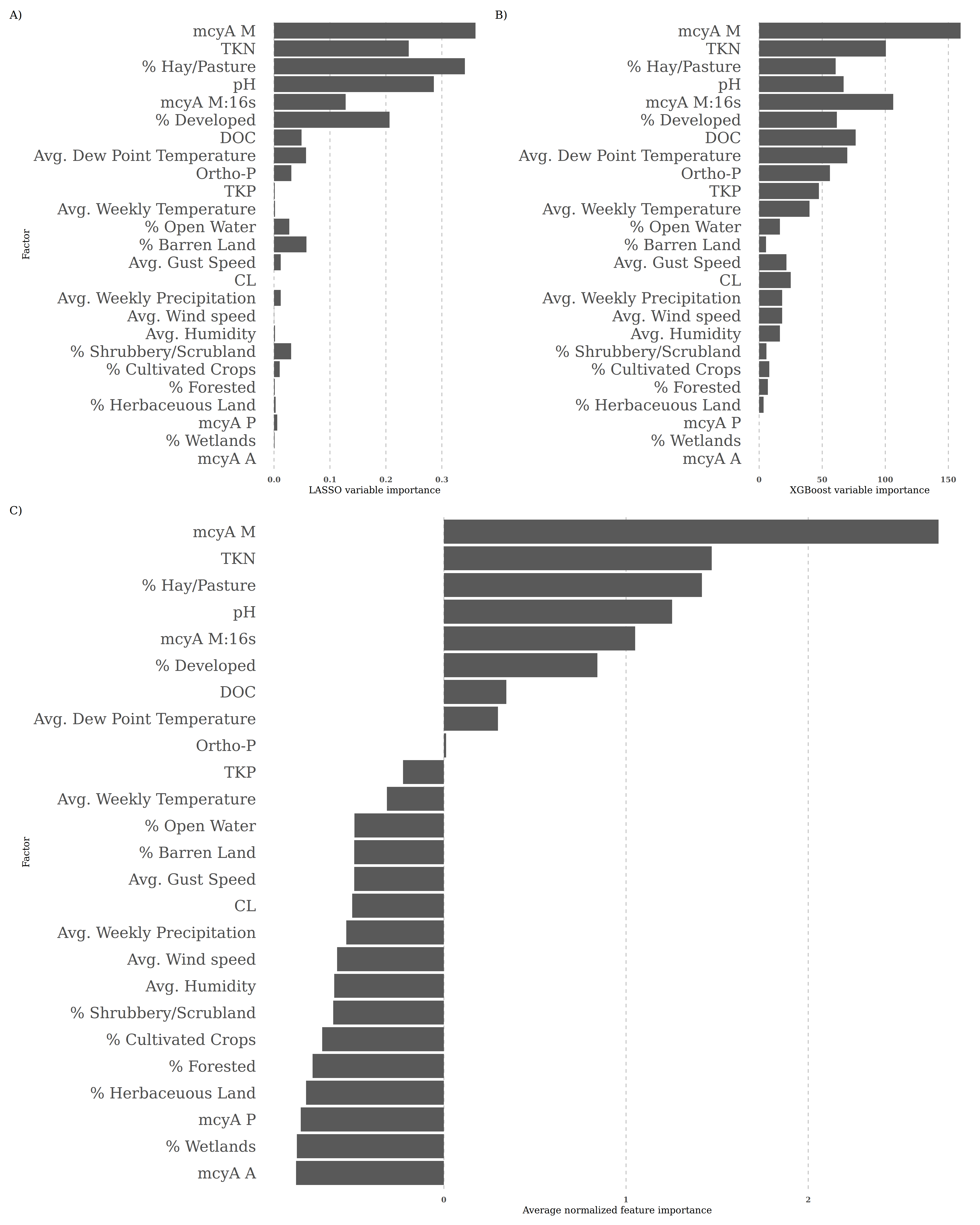
- XGBoost and LASSO both assign feature importance scores to the features used in the model. For each model type, we calculated the average feature importance score for each feature (Figures A and B below).
- We calculated an average normalized importance (ANI) by first normalizing the scores within each model type, then taking the mean of the importance scores for each feature (Figure C below).
- These feature importance scores measure how predictive of harmful algal bloom status each feature is. Because normalizing centers scores on zero, anything with an ANI greater than 0 has greater than average importance. These are the features we use in our downstream analysis.
Feature selections scores. Click here to see the full-size image.
The distribution of hazardous to non-hazardous samples is incredibly lopsided: after cleaning and preparing the data, only 70 samples of 1473 total samples (or less than 5%) were considered hazardous, which is is a class imbalance of 21 to 1. We tried some different strategies to address this.
- Oversampling the minority class using
themis::step_smoteto generate synthetic hazardous samples. There are some definite concerns with generating so many samples of the minority class when the class imbalance is so big, such causing the model to overfit the training set or introducing a lot of noise into the minority class. - Undersampling the majority class using
themis::step_downsample. While it felt like a waste to throw away so much data to even out the class distributions, doing so might lead to learning both classes evenly during training.
The aggregated results of the different sampling strategies are:
Averaging all the models together (explained further below), we see that the oversampling strategy typically performed better across the board. There is an argument to be made to using downsampling: while ROC AUC was comparable between the two strategies, downsampling might be preferable due to decreased data set size and to prevent overfitting during model training. However, the improvement in specificity using oversampling (representing roughly 4 additional correct guesses) is significant enough, and our interest in correctly predicting the the hazardous cases is that much higher than in overall performance, that oversampling (in general) is the better choice.
Note that this analysis is on sampling strategies as a whole averaged over all models.
Since the classes were so imbalanced, accuracy was clearly a poor choice here - any model that just predicts that there wouldn't be a harmful algal bloom would achieve 95% accuracy. Thus, we relied on ROC AUC and specificity in order to pick our best performing models, though we also recorded sensitivity and accuracy as well. In addition, we used a "naive" prediction model as a baseline which predicted next week's hazard status to be the current week's. For example, if week n was non-hazardous, then the naive model predicted that week n + 1 would also be safe.
Here are the results of the tuned model on the testing set, separated by model type and sampling strategy:
XGBoost performed well overall, with some sort of XGBoost model achieving the best scores over all the metrics. Since ROC AUC and Specificity were our metrics of interest, the downsampled XGBoost appears to be the model of choice for use in actual prediction.
The oversampled logistic regression is another choice worht considering, especially because it can be considered a simpler model while still achieving the same specificity and comparable ROC AUC. However, the accuracy and sensitivity are "significantly" lower, and even though predictions on the non-hazardous class are not as valuable for our study, there are real-world economic consequences for predicting false negatives (ie, predicting that a beach would experience a hazardous event when it does not) resulting from closures of lakes and beaches to recreational activity.
While the XGBoost models did perform well on our testing set, the sample size was only 14 hazardous samples. We next attempted ensemble modeling in order to boost all of the performance metrics. We created several ensemble models in order to improve the predictions. The candidates for the ensemble models were those models that performed the best in each of ROC AUC, accuracy, sensitivity, and specificity. Specifically, we used the over- and undersampled XGBoost models and the oversampled logistic regression. Our four ensemble models were:
- Blended predictions maximizing ROC AUC. This was constructed using the
stackspackage in R. - Blended predictions maximizing specificity, using
stacksas above. - Soft voting using the average class probability from the three models.
- Hard voting by taking the majority class vote for the member models.
Performance metrics for the different strategies:
According to our requirements for a high specificity and high ROC AUC, the hard voting strategy is the best candidate for implementation.
Getting the land use data and the climate data might not always be possible. For example, perhaps land use data is not available for a particular location (or may just be out of date), or climate data is just not available. To see how much their inclusion helps the models, we ran our ensemble model on the important features three more times: without climate data, without land use data, and without either. This implicitly puts more weight on the biologic and chemical data.
After retraining the models from, we got the following results:
The model trained with all of the variables in the previous step is in the first row, and we see that it achieves the highest ROC AUC and specificity, and is tied for highest accuracy. More specifically, since we are more concerned with specificity here, the margin of improvement by including all the variables shows that the inclusion of the climate and land use data is probably worth the trouble.
After cloning the repo, restore the conda environment by doing:
mamba env create -f environment.yml
Then, activate the environment:
conda activate hab_prediction
You can then run the pipeline with:
snakemake -c 4
(You can also do snakemake -c 1 to use fewer cores.)
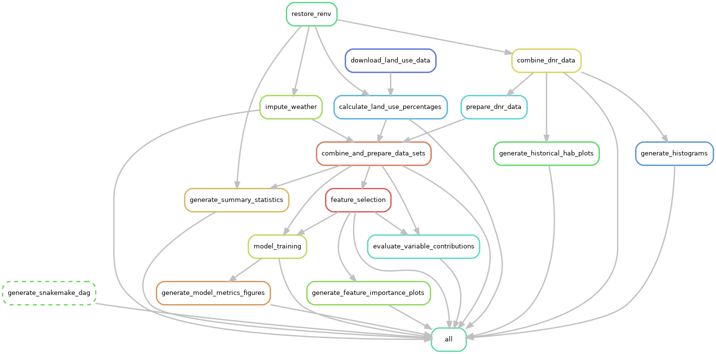
This will restore the R environment, regenerate all the figures, and render the website.


