Intro to SQL for Querying Databases

Author: Michele Tobias

This workshop teaches the basics of (non-spatial) SQL using DB Browsesr and SQLite. This workshop provides an overview of the utility and base SQL commands for working with data in a relational database. We’ll focus on querying data to get to know a database and answer questions, and combining data from separate tables.

Goals

After this workshop learners should be able to:

Perform common SQL commands including sorting, filtering, calculating values, aggregating, combining data, and basic data cleaning (i.e. replace missing values).
Combine commands to construct a query to answer a specific question.
Identify the benefits of working with SQL.
Access additional resources for using SQL in other software like R.

Prerequisites

No prior programming experience is necessary. Bring your laptop with DB Browser installed (https://sqlitebrowser.org/) and running.

Concepts

What is a Relational Database?

A database is a set of data in tables that are related to each other in some way. That's it. It's just a collection of tables.

Ideally each table can be connected to another table by a column that both tables have that store the information to match up the rows. This column is called a key. For example, a key commonly used on campus is your student or employee ID number.

Let's look at an example dataset of fictional student data with data about courses, grades, and employment. Can we say anything about the relationship between course grades and employment based on this data?

Table: Student

ID	Name
123	Jane Smith
456	Maria Martinez
789	Paul Jones

Table: Courses

ID	Course	Grade
123	Calculus	A-
456	Calculus	A
789	Calculus	C+
123	Data Science	A-
456	Data Science	B
789	Data Science	B-

Table: Employment

ID	Position	Employer	HoursPerWeek
123	Student Assistant	University Research Lab	5
456	Customer Service	Alumni Center	5
456	Research Assistant	University Research Lab	15
789	Student Assistant	University Research Lab	10
789	Stock Room	Medical Supplier	20
789	Customer Service	Alumi Center	15

What is SQL?

SQL stands for "structured query language" and it's a language that allows you to ask questions of a database.

In the above example, it would be much easier to understand the relationships if we build a table aggregating and reshaping our data. SQL allows us to do that.

You're Already Doing This!

Researchers typically are already thinking about querying data.

Imagine you have a table about air quality data. It contains columns with measurements about various environmental properties such as the temperature, the level of ozone, and perhaps measurements of various particulates.

If you've ever subsetted data in R, for example, you've already done something similar to writing an SQL query! The R code subset(airquality, Temp > 80, select = c(Ozone, Temp)) becomes SELECT Ozone, Temp FROM airquality WHERE Temp > 80 in SQL.

In Excel, you might sort your whole spreadsheet on the Temp column, then copy all of the rows that are greater than 80, and paste them into another tab. You might remove all the other columns except for the Ozone and Temp columns. You might have also used the cell highlighting tools to change the color of the cells based on the Temp column just to see which cells meet your criteria.

Why do you want to learn to work with databases and SQL?

Efficiency
- Write a few lines of code rather than lots of manual data manipulation
- SQL is meant for data manipulation
Reproducibility
- save queries as a record of your workflow
- re-run code with updates
Work with large amounts of data
- Typically faster to run a process in a database than in a spreadsheet
- Store lots of data (compare with Excel's row limits)
Data management
- One database file stores many, many tables which is represented as one file in your file browser
- Write a query instead of making a new files or tabs

What makes this challenging?

If you currently work in a graphical user interface (GUI), you might be used to being able to see your data, have tools with guided interfaces, and seeing the results of your processing immediately. These aren't things you get with a typical database manager tool, however, you will get used to the typical workflow and seeing everything won't be so necessary.

Getting Setup

Install the Software

We'll be using DB Browser, a free, open source, graphical interface for working with SQL databases that works on all major computing operating systems. Installers are available on their Downloads Page. If you do not have install permissions on your computer, the Portable App version may work without administrator permissions.

Download the Workshop Data

The data is available on Michele's Workshop Data Box Drive.
Dismiss the banner that might pop-up at the top of the webpage directing you to log-in (you don't need to log-in or have an account to download the data).
Click the Download button in the upper right corner to download all the data in one zipped file.
Save the data where you can find it easily, then unzip the folder.

Understanding the Data

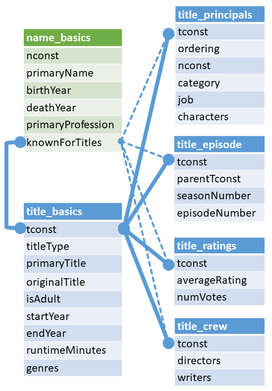
For this workshop, we'll be working with some data from IMDB (Internet Movie Database). You can get updated data on the IMDB Datasets Page. The diagram below outlines the relationships between the data in the tables that make up the database. Notice how information about the movie and TV show titles is all connected by the tconst column. This is a key, a unique identifier for each title. The cast and behind-the-scenes people also have a key - it's called nconst.

I've already pre-processed the data so that it's easier to import into your SQL database and small enough to work reasonably well in a workshop, so if you get new data, you'll have to unzip the downloaded data, and save it as a csv file before proceeding. The full IMDB database is rather large and growing daily, so feel free to explore it, but know that some of the tables are over 2GB in their original state.

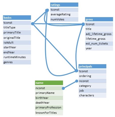
The data we'll be working with is an extract from the IMDB dataset from Oct. 18, 2019. Specifically, we'll be looking at the top 200 grossing movie titles and related data. Here is a diagram of the data we'll be working with:

Notice how most of the tables can be connected with the tconst column. The contents of most of the tables are described on IMDB's database documentation page. The data in the gross table are described by BoxOffice Mojo, a division of IMDB.

Hands On

Start DB Browser

Start the DB Browser for SQLite program in the way you usually start new programs on your computer. For example, on Windows 10, I typically search for the program name in the search box.

Create a New Database

First, let's create a new database to store our data. Remember that a database is like a container that holds related tables.

Click on the New Database button
Navigate to where you'd like to save your database. I'd suggest putting it in the folder where you're keeping your workshop data.
In the File name box, call your database "imdb", and then click Save. You can dismiss the window that pops up to Edit table definition. We'll load data in a different way.

Now we have an empty database called imdb.db.

Import the Data into a Database

Let's load the first data table:

From the File menu, select Import, and then Table from CSV....
Navigate to where you saved your workshop data and select basics.csv and click the Open button. A new dialog window should pop up now.
In the Table name field, you could change your table name. This is handy because if your data file is named something complicated, you can name it something easier to type here. Let's leave the name as basics.
Check the box next to Column names in first line because our data has headers.
Notice that the preview of the table does not look right. The column names are not what we would expect for a table of information about actors. Change the Field separator drop-down menu to Tab. Notice the change in the preview. That looks better!
Change the Quote character to the blank space on the drop-down menu. The quotes that appear in the data do not indicate that something is text, but rather are used in a more literary sense. If we don't change this, our data import will fail (your instructor learned this from personal experience).
We can leave the Encoding as UTF-8. Note: when you load your own data, if you get odd characters in your preivew, check to see what your character encoding should be. Trim fields removes extra spaces.
Click the OK button when everything looks as you would expect.

Repeat the process with the gross.csv, name.csv, principals.csv, and ratings.csv files.

The DB Browser Interface

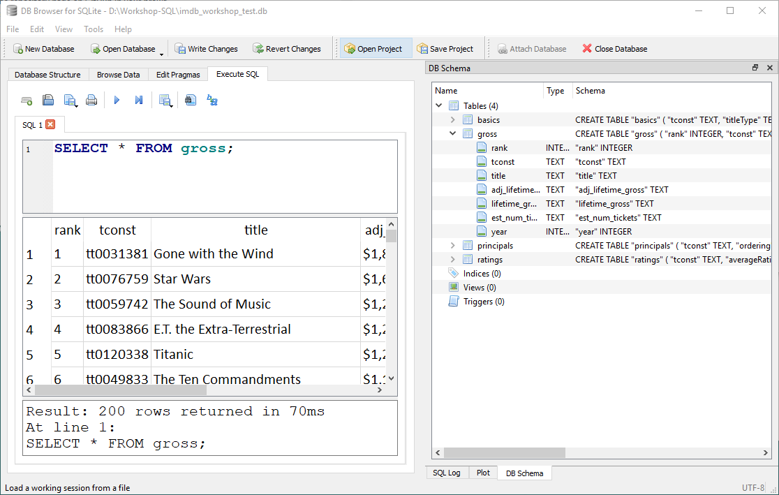
DB Browser has a number of tabs and tools to help you interact with your data. We'll be mainly working with the Execute SQL tab, so go ahead and click on that tab. We'll write our queries in the top portion of the interface, the results will be returned to the middle pannel, and messages will return to the bottom portion.

Notice also the DB Schema panel on the right side of the window. It should show all of the tables you've added. If you click on the > symbol next to the table name, the interface will expand a list of the columns in your table.

Viewing Data

Anatomy of a SELECT Statement

We're ready to write our first queries! The most common query you'll use is the SELECT statement. In it's most basic form, it shows you the data in a table, but you can add option to customize the view you get back. Let's try! Type this query into the query box:

SELECT * FROM gross;

Now click the Execute all button.

This query asks the database to select everything (* means "everything") from the table gross. It ends with a semicolon to tell the database that this is the end of our request.

SELECT 
* 
FROM 
gross;

The above query does exactly the same thing as the first one, hence the need for the end of query indicator. We can use new lines to help us organize large queries to make them easier to read.

Capitolization in queries follows some general rules:

Commands are in all caps
Table names and column names are all lowercase

Will the query work if you don't do this? It depends on the interface you're using, but generally it will work. DB Browser doesn't mind either way. In the text of this workshop, I will try to be consistent and use the proper form.

Selecting Columns

What if we don't want to see all of the columns in the table? We can ask for just the columns we want to see. Let's get the title, the year the movie came out, and the ajusted lifetime gross income:

SELECT title, year, adj_lifetime_gross 
FROM gross;

Ordering Results

What if I want to see them in order of the year they were made?

SELECT title, year, adj_lifetime_gross 
FROM gross
ORDER BY year;

CHALLENGE: How would I order the table by the adjusted lifetime gross income?

The default order by option sorts in ascending order. We can sort in descending order to get the top grossing movies first by adding the DESC parameter:

SELECT title, year, adj_lifetime_gross 
FROM gross
ORDER BY adj_lifetime_gross DESC;

Limiting Number of Rows

Our database has the top 200 movies. What if we just want a table of the top 10? We can use the LIMIT command to reduce the number of rows the query returns.

SELECT title, year, adj_lifetime_gross 
FROM gross
ORDER BY adj_lifetime_gross DESC
LIMIT 10;

Calculating Values

Let's investigate the earnings of these movies.

In their current state, the numbers in the adj_lifetime_gross column are hard to compare. We can add mathematical operators and numbers to the column name to perform the calculation. Let's calculate the adjusted lifetime gross column in billions of dollars (9 zeros):

SELECT title, year, adj_lifetime_gross/1000000000
FROM gross;

Renaming/Aliasing Columns

Doing calculations is helpful for visualizing data, but the default column name is not always easy to read or interpret. We can rename columns in the text of our query. This is handy if you're planning to export this table for future use, especially if you're sending it to someone else. Let's rename our calculated column using the AS option.

SELECT title, year, adj_lifetime_gross/1000000000 AS gross_billions
FROM gross;

Commenting Queries

Sometimes we want to be able to write a comment, text that won't be interpreted by the interface as a part of the query. Any text that follows two dashes -- until the end of the line is a comment.

SELECT title, year, adj_lifetime_gross/1000000000 AS gross_billions -- 1 billion has 9 zeros
FROM gross;

Unique Values

In your data exploration, you might want to know which categories you're working with if you have a categorcal variable. Let's look at the principals table which contains the roles played in each movie.

REVEIW How would you see all the data in the principals table? I'll typically view all the data (adding a LIMIT parameter if it's a big one) before I write queries just to get a better feel for the information that's contained there.

I'm curious about how many different roles are used in the category field.

SELECT DISTINCT(category) 
FROM principals;

DISTINCT is a function that we can run on a column. In this case, the function returns a list of unique values from the column, so each item is only listed once.

Filtering Results

Now that we know what kinds of job rolls are listed in the principals table's category field, let's filter the table to look at the records for just one job type.

SELECT * 
FROM principals
WHERE category LIKE 'actor';

The WHERE option lets us specify a condition of the record to filter on. (For you spatially-minded folks, WHERE does not inherently mean a location.)

What does LIKE mean? Why not use = ? For text-based data (non-numeric data), the comparison operators are different. You can think of LIKE for text as being about the same as = for numeric data.

The above query returns just the actors, so male people in an acting role. By now, you probably can figure out how to get filter for actresses, or female people in an acting role, BUT how can we get both? We can ask WHERE to meet multiple conditions using either OR (for where a record can match either of two conditions) or AND (when a record must match both conditions). Let's get both actors and actresses:

SELECT * 
FROM principals
WHERE 
category LIKE 'actor' 
OR category LIKE'actress';

Wildcard Matching

There is another way to write this query. Because our categories are similar, we can use a wildcard - % in SQL - to indicate that we want to match the beginning of the word, but the end is allowed to vary. Let's take a look:

SELECT * 
FROM principals
WHERE 
category LIKE 'act%';

You can also use the wildcard character at the beginning of the word as well. The % wildcard is useful for fairly simple situations. You can also use regular expressions to match in more complicated situations. Read more about using regular expressions here.

Aggretating Data

We've just looked a number of ways to filter data, but now let's look at some ways to aggregate data.

Count

It probably won't surprise you that we can count the number of records or that this particular query returns the number 200:

SELECT COUNT(tconst) 
FROM ratings;

You might also suspect that you can add WHERE clause to this to get more information. Let's see how many movies in our dataset are rated better than or equal to 8.0:

SELECT COUNT(tconst) 
FROM ratings
WHERE averageRating >= 8.0;

We could also find out how many are greater than or equal to 8.0 but less than 8.5 using an AND:

SELECT COUNT(tconst) 
FROM ratings
WHERE averageRating >= 8.0 AND averageRating < 8.5;

Average

Averaging is another function we can use to aggregate data. Let's find the average adjusted lifetime gross of our top 200 movies:

SELECT AVG(adj_lifetime_gross) 
FROM gross;

CHALLENGE: How many billions of dollars is this?

Sum

We can also sum our data. Let's find the sum of the adjusted lifetime gross of our movies;

SELECT SUM(adj_lifetime_gross) FROM gross;

Grouping Data

So now you've seen several functions working on a single column. But we sometimes want to summarize our data in more sophisticated ways. Let's see what grouping can do for our data. Let's make a table that counts the number of records in our principals table and summarizes it by the category (actress, actor, composer, etc.):

SELECT category, COUNT(nconst) 
FROM principals
GROUP BY category;

Notice here how we asked for two columns - the category and the count of the name ID. This makes the resuts of the COUNT funtion easier to understand.

Having

HAVING is just like WHERE but it specifically works with grouping data. Perhaps we're only interested in the categories of principals that have more than 100 people. Let's see what that looks like:

SELECT category, COUNT(nconst) 
FROM principals
GROUP BY category
HAVING COUNT(nconst) > 100;

Now we've seen how we can use functions to aggregate data and how grouping data can help us make meaningful tables. There are, of course, other functions available in SQL and we can't go over all of them here, but now you've seen how they work and can apply your knowledge to new functions you find.

Joins

Joining tables allows us to combine information from two tables into a new table. Both tables need to have information in common to be able to match up the records in each table, called a key. For example, in the introduction, a student ID number links information in our tables. In our IMDB data, the tconst variable links information in most of our tables.

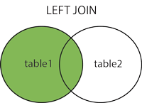
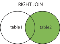
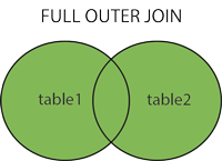
SQL has 4 kinds of joins:

The above images come from the W3Schools' SQL join page, an excellent resource for learning more about SQL.

What kinds of joins are there?

JOIN: Returns records that have matching values in both tables; sometimes called an "inner join" because it gets you what's in the middle of the Venn diagram.
LEFT (OUTER) JOIN: Returns all records from the left table, and the matched records from the right table; the "left" table is the first table you write in the query.
RIGHT (OUTER) JOIN: Returns all records from the right table, and the matched records from the left table; the "right" table is the second table you write in the query or the "join" table. Not currently supported in DB Browser.
FULL (OUTER) JOIN: Returns all records when there is a match in either left or right table; nulls are generated in the table when a row in one table doesn't have a match in the other table. Not currently supported in DB Browser.

A join is a special kind of select statement. We start in just the same way: SELECT the columns we want in the output (using table.column syntax to indicate which table each column comes from). Then we have the FROM statement to tell it which table to start with (this is our "left" table). Then we need our JOIN statement to say which table should get joined (this is our "right" table), and finally, we have to say which columns the join should be based on with either ON (for any columns) or USING (when the column names match... although ON also works in this case and it's what I always remember). Let's try a join to see how this works:

SELECT  basics.tconst, gross.title, gross.year, basics.runtimeMinutes 
FROM basics
JOIN gross
ON basics.tconst = gross.tconst;

We can use the USING clause when the join columns from both tables have the same name:

SELECT  basics.tconst, gross.title, gross.year, basics.runtimeMinutes 
FROM basics
JOIN gross
USING (tconst);

CHALLENGE: Can you make a table that contains the movie names and all the principal jobs for each movie?

Don't look, but here's one solution:

SELECT  basics.*, principals.* 
FROM principals
LEFT JOIN basics
USING (tconst);

Occasionally, you can write a join-like query using a WHERE clause (SELECT columns FROM table WHERE table_a.col = table_b.col). I would suggest that this is ok, but the real power in writing SQL statements is in precision, so writing out a proper join is a good idea.

Saving Queries

Normally, we don't need to save a bunch of tables because we can always run a query to get the information, but sometimes we might want to save a query as a table or a view if the contents of that query is something we plan to use repeatedly. Use this new power sparingly to keep your database organized.

We have two options to save a query as a table-like object. One option is to make a new table. This is a separate set of data stored in table format, just like the tables you've been working with. The other option is to make a view. A view is a virtual table. The data in a view comes from other tables. You can think of this as a query that automatically runs itself and will updat if the tables it queries changes. A view behaves otherwise just like a table - you can use it in pretty much the same way you would a table. The only major difference is that a view, because it is updating from other tables, is not able to be edited.

Let's write a fairly complicated query that we might want to keep around. This one joins 3 tables into one:

SELECT principals.nconst, name.primaryName, principals.category, principals.job, principals.characters, basics.tconst, basics.primaryTitle, basics.startYear, basics.runtimeMinutes
FROM principals
LEFT JOIN basics USING (tconst)
JOIN name on principals.nconst = name.nconst;

If we want to make a table out of this query, we just need to add CREATE TABLE our_new_table_name AS in front of the query (adding in our own table name, of course). This is what it looks like:

CREATE TABLE principals_movies AS
SELECT principals.nconst, name.primaryName, principals.category, principals.job, principals.characters, basics.tconst, basics.primaryTitle, basics.startYear, basics.runtimeMinutes
FROM principals
LEFT JOIN basics USING (tconst)
JOIN name on principals.nconst = name.nconst;

In much the same way we made the new table, we can make a view:

CREATE VIEW principals_movies_view AS
SELECT principals.nconst, name.primaryName, principals.category, principals.job, principals.characters, basics.tconst, basics.primaryTitle, basics.startYear, basics.runtimeMinutes
FROM principals
LEFT JOIN basics USING (tconst)
JOIN name on principals.nconst = name.nconst;

You might notice now that your new view is the the views section of your DB Schema panel.

Normally you wouldn't need to make both a view and a table, but this is a workshop and you need to see how to do all the important things.

Data Management

Fix Mistakes with UPDATE

Now you might have noticed that our new table principals_movies has some funny characters. The IMDB database uses the characters \n instead of NULL or NA. The good news is that we can fix this fairly easily, but we need to be careful. It's challenging to undo something in a database so we want to be sure we're doing it right.

First, I construct a SELECT statement to make sure I know how to get the records I want to update:

SELECT * FROM  principals_movies
where job LIKE '\N';

This looks good because it returns just the records where the jobs column is \N so I know I can update that column:

UPDATE principals_movies
SET job = NULL
where job LIKE '\N';

This query specifically targets just the job column and replaces whatever value is there with the one I want (NULL) if the condition is met in the WHERE clause. It leaves the other values alone. If I remove the WHERE clause, it will set the whole column to NULL overwriting data I want to keep, so proceed with caution. Also note, that because we're working on a table that we made and aren't changing the original tables, we can always remake the table we're working on if we make a mistake. It's always a good idea to have back-up copies of data in case you make a mistake.

CHALLENGE: Write a query that also removes the \N characters from the characters column.

Add & Populate a Column

Sometimes we want to make a new column and add data into it. Let's make a new column called acting_role and populate it with a 1 if the category is actor or actress and 0 if it's something else.

First we add a column and set the default value to 0:

ALTER TABLE principals_movies
ADD acting_role INTEGER DEFAULT 0;

Note that the DEFAULT argument is optional, but if you leave it blank, it will make the default value NULL. Now we update the column to be 1 where the category is actor or actress:

UPDATE principals_movies
SET acting_role = 1
WHERE category LIKE 'act%';

Conclusion

We covered a wide variety of SQL processes you might need in setting up a database and querying data. Did we cover everything you might need to know? Of course not. It's only a 2 hour workshop and SQL is a big language. I highly encourage you to look at the resources below to learn more and expand your SQL skills. I also welcome pull requests and submitting issues for typo fixes or ideas for additional content.

Resources

W3Schools SQL Materials - This is an excellent reference for SQL syntax with a fun "try it yourself" feature.

Sofware Carpentry's SQL Novice Workshop

Clark Fitzgeralds & Nick Ulle's SQL Workshop

Michele Tobias' Spatial SQL Workshop

Working with SQL databases and queries in R:

ponteviti/Workshop-SQL