To get started we will first dwell into the atmosphere of the sun and checkout what's hot there 😉

The atmosphere of the sun is composed of several layers, mainly the photosphere, the chromosphere and the corona. It's in these outer layers that the sun's energy, which has bubbled up from the sun's interior layers, is detected as sunlight.

The lowest layer of the sun's atmosphere is the photosphere. It is about 300 miles (500 kilometers) thick. This layer is where the sun's energy is released as light. The photosphere is marked by bright, bubbling granules of plasma and darker, cooler sunspots, which emerge when the sun's magnetic field breaks through the surface. The bumps are the upper surfaces of the convection current cells beneath; each granulation can be 600 miles (1,000 kilometers) wide. As we pass up through the photosphere, the temperature drops and the gases, because they are cooler, do not emit as much light energy. This makes them less opaque to the human eye. Therefore, the outer edge of the photosphere looks dark, an effect called limb darkening that accounts for the clear crisp edge of the sun's surface. The photosphere is also the source of solar flares: tongues of fire that extend hundreds of thousands of miles above the sun's surface. Solar flares produce bursts of X-rays, ultraviolet radiation, electromagnetic radiation and radio waves.
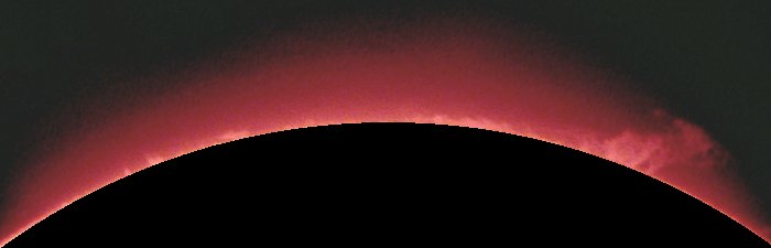
The next layer is the chromosphere. The chromosphere emits a reddish glow as super-heated hydrogen burns off.The temperature rises across the chromosphere from 4,500 degrees Kelvin to about 10,000 degrees Kelvin. The chromosphere is thought to be heated by convection within the underlying photosphere. As gases churn in the photosphere, they produce shock waves that heat the surrounding gas and send it piercing through the chromosphere in millions of tiny spikes of hot gas called spicules. Each spicule rises to approximately 3,000 miles (5,000 kilometers) above the photosphere and lasts only a few minutes. Spicules may also follow along magnetic field lines of the sun, which are made by the movements of gases inside the sun. But the red rim can only be seen during a total solar eclipse. At other times, light from the chromosphere is usually too weak to be seen against the brighter photosphere.

The third layer of the sun's atmosphere is the corona. It can only be seen during a total solar eclipse as well. It
appears as white streamers or plumes of ionized gas that flow outward into space. Temperatures in the sun's corona
can get as high as 3.5 million degrees F (2 million degrees C). As the gases cool, they become the solar wind.
There is one interesting thing about corona: The surface of the sun is almost 10,000 degrees Fahrenheit. That’s
really hot. But the sun’s corona is over 200 times hotter—millions of degrees Fahrenheit. That’s like the actual
flame of a fire being 200 times colder than the air around that fire.
Why would the area around a hot burning mass be hotter than something that is actually closer to the source of heat?
And if the corona is so hot, then why doesn’t it heat up the sun’s surface to a similar temperature?
Well, the truth is that nobody knows for sure. Lots of scientists are hard at work trying to figure out the answer.
One potential explanation is magnetic forces. All that superheated gas in the sun core creates a strong magnetic
field—like Earth’s magnetic field, but a whole lot stronger and more chaotic. Some scientists think that it is this
magnetic field that gives the sun’s corona energy.If that were true, then powerful magnetic waves would be causing
atoms in the gas surrounding the sun to move very quickly. The faster the atoms in something move, the hotter it is.
That’s all heat is—moving atoms.
It’s very hard to study the sun, and scientists are still not entirely sure how magnetic force could produce heat,
or why the surface of the sun is not heated by the hot corona. But that’s the great thing about science—there’s
always some big mystery just waiting to be solved.
The high temperature of the Sun's corona gives it unusual spectral features, which led some in the 19th century to
suggest that it contained a previously unknown element, "coronium". Instead, these spectral features have since been
explained by highly ionized iron (Fe-XIV). Bengt Edlén, following the work of Grotrian (1939), first identified the
coronal spectral lines in 1940 (observed since 1869) as transitions from low-lying metastable levels of the ground
configuration of highly ionised metals (the green Fe-XIV line at 5303 Å, but also the red line Fe-X at 6374 Å).
These high stages of ionisation indicate a plasma temperature in excess of 1,000,000 kelvin, much hotter than the
surface of the sun.
Light from the corona comes from three primary sources, from the same volume of space.
The K-corona (K for kontinuierlich, "continuous" in German) is created by sunlight scattering off free electrons;
Doppler broadening of the reflected photospheric absorption lines spreads them so greatly as to completely obscure
them, giving the spectral appearance of a continuum with no absorption lines.
The F-corona (F for Fraunhofer) is created by sunlight bouncing off dust particles, and is observable because its
light contains the Fraunhofer absorption lines that are seen in raw sunlight; the F-corona extends to very high
elongation angles from the Sun, where it is called the zodiacal light.
The E-corona (E for emission) is due to spectral emission lines produced by ions that are present in the coronal
plasma; it may be observed in broad or forbidden or hot spectral emission lines and is the main source of
information about the corona's composition.
The corona is not always evenly distributed across the surface of the sun. During periods of quiet, the corona is more or less confined to the equatorial regions, with coronal holes covering the polar regions. However, during the Sun's active periods, the corona is evenly distributed over the equatorial and polar regions, though it is most prominent in areas with sunspot activity. The solar cycle spans approximately 11 years, from solar minimum to the following minimum. Since the solar magnetic field is continually wound up due to the faster rotation of mass at the sun's equator (differential rotation), sunspot activity will be more pronounced at solar maximum where the magnetic field is more twisted. Associated with sunspots are coronal loops, loops of magnetic flux, upwelling from the solar interior. The magnetic flux pushes the hotter photosphere aside, exposing the cooler plasma below, thus creating the relatively dark sun spots.
Since the corona has been photographed at high resolution in the X-ray range of the spectrum by the satellite Skylab in 1973, and then later by Yohkoh and the other following space instruments, it has been seen that the structure of the corona is quite varied and complex: different zones have been immediately classified on the coronal disc. The astronomers usually distinguish several regions, as described below.
Active regions are ensembles of loop structures connecting points of opposite magnetic polarity in the photosphere, the so-called coronal loops. They generally distribute in two zones of activity, which are parallel to the solar equator. The average temperature is between two and four million Kelvin, while the density goes from 109 to 1010 particle per cm3.
Large-scale structures are very long arcs which can cover over a quarter of the solar disk but contain plasma less dense than in the coronal loops of the active regions. The large-scale structure of the corona changes over the 11-year solar cycle and becomes particularly simple during the minimum period, when the magnetic field of the Sun is almost similar to a dipolar configuration (plus a quadrupolar component).
Filament cavities are zones which look dark in the X-rays and are above the regions where Hα filaments are observed in the chromosphere. They were first observed in the two 1970 rocket flights which also detected coronal holes. Filament cavities are cooler clouds of gases (plasma) suspended above the Sun's surface by magnetic forces. The regions of intense magnetic field look dark in images because they are empty of hot plasma.
The matter in the external part of the solar atmosphere is in the state of plasma, at very high temperature (a few million Kelvins) and at very low density. According to the definition of plasma, it is a quasi-neutral collection of particles which exhibits a collective behaviour.
The composition is the same as the one in the Sun's interior, mainly hydrogen, but completely ionized, thence protons and electrons, and a small fraction of the other atoms in the same percentages as they are present in the photosphere. Even heavier metals, such as iron, are partially ionized and have lost most of the external electrons. The ionization state of a chemical element depends strictly on the temperature and is regulated by the [Saha equation ](https://en.wikipedia.org/wiki/Saha_ionization_equation).
The corona behaves like a gas which is very hot but very light at the same time: the pressure in the photosphere is usually only 0.1 to 0.6 Pa in active regions, while on the Earth the atmospheric pressure is about 100 kPa, approximatively a million times higher than on the solar surface. However it is not properly a gas, because it is made of charged particles, basically protons and electrons, moving at different velocities. Supposing that they have the same kinetic energy on average (for the equipartition theorem), electrons have a mass roughly 1800 times smaller than protons, therefore they acquire more velocity. Metal ions are always slower. This fact has relevant physical consequences either on radiative processes (that are very different from the photospheric radiative processes), or on thermal conduction. Furthermore, the presence of electric charges induces the generation of electric currents and high magnetic fields. [Magnetohydrodynamic waves](https://en.wikipedia.org/wiki/Magnetohydrodynamics) can also propagate in this plasma, even if it is not still clear how they can be transmitted or generated in the corona.
The corona emits radiation mainly in the X-rays, observable only from space. The plasma is transparent to its own radiation and to that one coming from below, therefore we say that it is optically-thin. The gas, in fact, is very rarefied and the photon mean free-path overcomes by far all the other length-scales, including the typical sizes of the coronal features. Different processes of radiation take place in the emission, due to binary collisions between plasma particles, while the interactions with the photons, coming from below; are very rare. Because the emission is due to collisions between ions and electrons, the energy emitted from a unit volume in the time unit is proportional to the squared number of particles in a unit volume, or more exactly, to the product of the electron density and proton density.
After having given a brief idea of Corona and its properties, now I will get to more details about the electron density profile and the refractive index of the corona.
In the normal background corona, we will adopt the conventional Bambauch-Allen model for the radial distribution of electron density.
To start with, I modelled trajectory of a ray propagating through a rectangular slab of a given refractive index. This is the code which plots the trajectory of ray given a refractive index through a rectangular slab.
Here is the code for the same :
import numpy as np
import simpy
import matplotlib.pyplot as plt
import sys

sys.setrecursionlimit(1500)

no_of_iterations = 1000
vec_x = np.arange(no_of_iterations)
in_angle  = np.pi*25.0/180.0                                 #incident angle
in_height = 10                             #The value of y co-ordinate where the ray hits the medium
vec_y = np.zeros(no_of_iterations)
r_index = np.ones(no_of_iterations)

for i in range(1,1000) :
	r_index[i] = r_index[i]/(1+ float(i)/1000.0)      #set the refractive index function here.


r_index[0] = 1                               #refractive index of outer medium


def ang_of_incidence(n):                     #decides the angle of refraction for the next iteration step
    if n == 1:
    	incident_ang = np.sin(in_angle)*(r_index[0]/r_index[1])
        return incident_ang
    else:
    	incident_ang = (r_index[n-1]/r_index[n])*ang_of_incidence(n-1)
        return  incident_ang

def path_eq(n):                               #trajectory of ray

	if n  == 0:
		vec_y[n] = in_height
		return vec_y

	else:
		vec_y[n] = path_eq(n-1)[n-1] + np.tan(np.arcsin(ang_of_incidence(n)))
		return vec_y

def get_slope(n):
    print('slope : ' , (180/np.pi)*np.arcsin(ang_of_incidence(n)))

get_slope(50)


plt.plot(vec_x, path_eq(no_of_iterations-1))
plt.xlabel('x')
plt.ylabel('y')
plt.show()
For the refractive index profile taken as example the output is as follows:

Further details can be found here: Click Here